Recurrence after treatment of arteriovenous malformations of the head and neck

Do-Thi Ngoc Linh; Lam Khanh; Le Thanh Dung; Nguyen Hong Ha; Tran Thiet Son; Nguyen Minh Duc; Do-Thi Ngoc Linh; Lam Khanh; Le Thanh Dung; Nguyen Hong Ha; Tran Thiet Son; Nguyen Minh Duc

doi:10.3934/medsci.2022003

AIMS Medical Science

2022, Volume 9, Issue 1: 9-17. doi: 10.3934/medsci.2022003

Previous Article Next Article

Research article

Recurrence after treatment of arteriovenous malformations of the head and neck

1.
Department of Maxillofacial and Plastic Surgery, Viet Duc Hospital, Hanoi, Vietnam
2.
Department of Plastic and Reconstructive Surgery, Hanoi Medical University, Hanoi, Vietnam
3.
Department of Radiology, 108 Military Central Hospital, Hanoi, Vietnam
4.
Department of Radiology, Viet Duc Hospital, Hanoi, Vietnam
5.
Department of Plastic Surgery, University of Medicine and Pharmacy, Hanoi National University, Hanoi, Vietnam
6.
Department of Radiology, Pham Ngoc Thach University of Medicine, Ho Chi Minh City, Vietnam
† These two authors contributed equally.

Received: 17 December 2021 Revised: 19 February 2022 Accepted: 24 February 2022 Published: 09 March 2022

Objective
Arteriovenous malformations (AVMs) are aggressive diseases with a high tendency to recur. AVM treatment is complex, especially in the anatomically difficult head and neck region. This study analyzed correlations between extracranial head and neck AVM presentations and the frequency of recurrence.

Methods
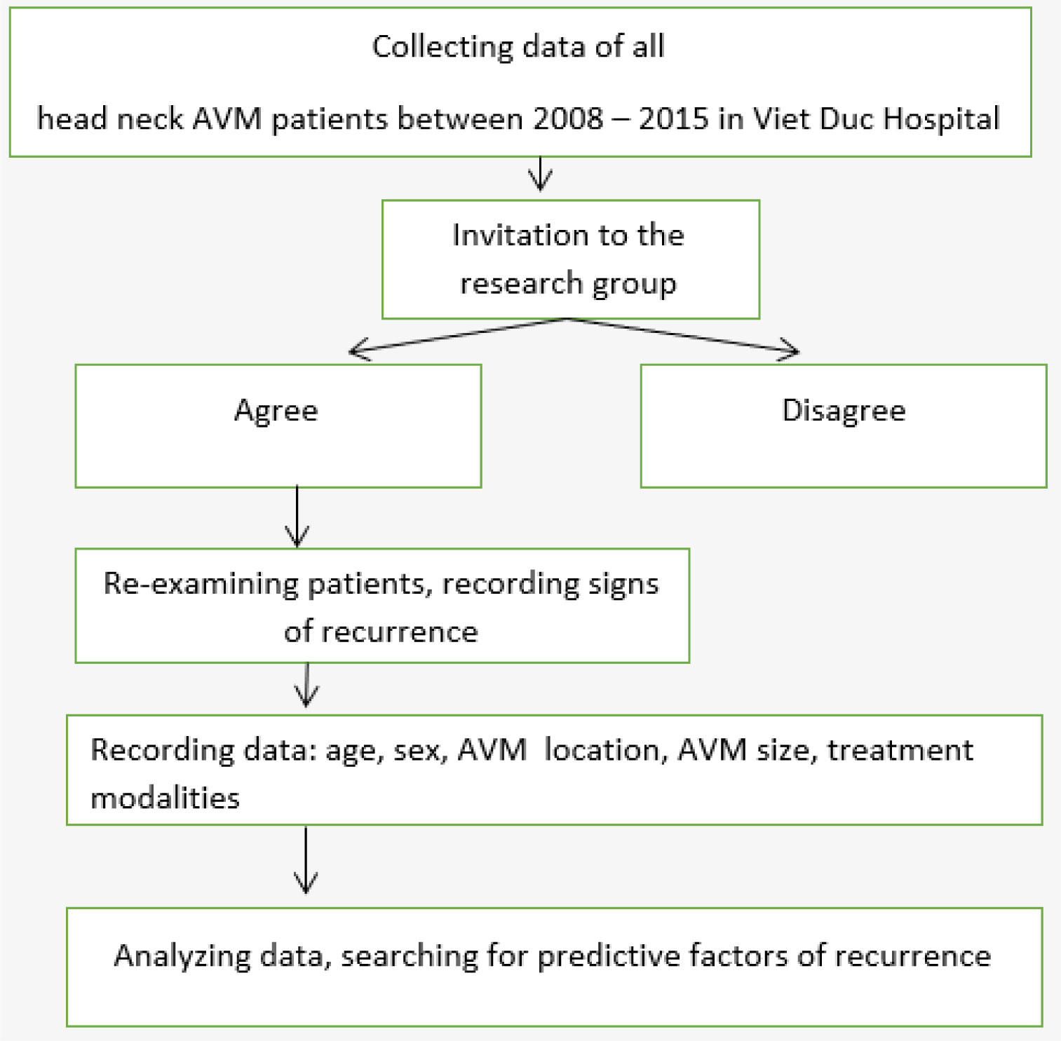
We retrospectively assessed AVM recurrence among 55 patients with head and neck AVMs treated with embolization and resection between January 2008 and December 2015. Recurrence was defined as any evidence of AVM expansion following embolization and resection. Patient variables, including sex, age, AVM size, AVM location, stage, and treatment modalities, were examined for correlations with the recurrence of head and neck AVMs. Statistical analysis was performed using SPSS 20.0.

Results
A total of 55 patients with at least 6 months of follow-up following AVM treatment with embolization and surgical resection were enrolled in this study. During follow-up, 14 of 55 patients experienced recurrence (the long-term recurrence rate was 25.5%). Sex, stage, AVM size, and treatment modality were identified as independent predictors of recurrence. Recurrence was less likely following the treatment of lower-stage or smaller lesions and did not correlate with age or location.

Conclusions
AVMs of the head and neck are among the most challenging conditions to manage due to a high risk of recurrence. Early and total AVM resection is the best method for preventing recurrence.
- arteriovenous malformations,
- embolization,
- surgery,
- recurrence,
- treatment outcome
Citation: Do-Thi Ngoc Linh, Lam Khanh, Le Thanh Dung, Nguyen Hong Ha, Tran Thiet Son, Nguyen Minh Duc. Recurrence after treatment of arteriovenous malformations of the head and neck[J]. AIMS Medical Science, 2022, 9(1): 9-17. doi: 10.3934/medsci.2022003

Related Papers:

Abstract

Objective

Arteriovenous malformations (AVMs) are aggressive diseases with a high tendency to recur. AVM treatment is complex, especially in the anatomically difficult head and neck region. This study analyzed correlations between extracranial head and neck AVM presentations and the frequency of recurrence.

Methods

We retrospectively assessed AVM recurrence among 55 patients with head and neck AVMs treated with embolization and resection between January 2008 and December 2015. Recurrence was defined as any evidence of AVM expansion following embolization and resection. Patient variables, including sex, age, AVM size, AVM location, stage, and treatment modalities, were examined for correlations with the recurrence of head and neck AVMs. Statistical analysis was performed using SPSS 20.0.

Results

A total of 55 patients with at least 6 months of follow-up following AVM treatment with embolization and surgical resection were enrolled in this study. During follow-up, 14 of 55 patients experienced recurrence (the long-term recurrence rate was 25.5%). Sex, stage, AVM size, and treatment modality were identified as independent predictors of recurrence. Recurrence was less likely following the treatment of lower-stage or smaller lesions and did not correlate with age or location.

Conclusions

AVMs of the head and neck are among the most challenging conditions to manage due to a high risk of recurrence. Early and total AVM resection is the best method for preventing recurrence.

Acknowledgments

This work was not supported by any funding.

Authors contributions

Study concept and design: DTNL, LK, TTS, and NMD; acquisition of data: DTNL, LK, TTS, and NMD; analysis and interpretation of data: DTNL, LK, TTS, and NMD; drafting of the manuscript: DTNL and NMD; critical revision of the manuscript: DTNL and NMD; statistical analysis: DTNL and TTS; study supervision: LK and TTS; and manuscript approval: DTNL, LK, LTD, NHH, TTS, and NMD.

Conflict of interest

All the authors declare that there are not biomedical financial interests or potential conflicts of interest in writing this manuscript.

References

[1]	Uller W, Alomari AI, Richter GT (2014) Arteriovenous malformation. Semin Pediatr Surg 23: 203-207. https://doi.org/10.1053/j.sempedsurg.2014.07.005
[2]	Pekkola J, Lappalainen K, Vuola P, et al. (2013) Head and neck arteriovenous malformations: Results of ethanol sclerotherapy. American J Neuroradiol 34: 198-204. http://doi.org:10.3174/ajnr.A3180
[3]	Mulliken JB, Fishman SJ, Burrows PE (2000) Vascular anomalies. Curr Probl Surg 37: 517-584. https://doi.org/10.1016/S0011-3840(00)80013-1
[4]	Mulliken JB, Burrows PE, Fishman SJ (2013) Mulliken and Young's vascular anomalies: Hemangiomas and malformations.Oxford University Press. https://doi.org/10.1093/med/9780195145052.001.0001
[5]	Kohout MP, Hansen M, Pribaz JJ, et al. (1998) Arteriovenous malformations of the head and neck: natural history and management. Plast Reconstr Surg 102: 643-654. https://doi.org/10.1097/00006534-199809010-00006
[6]	Liu AS, Mulliken JB, Zurakowski D, et al. (2010) Extracranial arteriovenous malformations: natural progression and recurrence after treatment. Plast Reconstr Surg 125: 1185-1194. https://doi.org/10.1097/PRS.0b013e3181d18070
[7]	Wu JK, Bisdorff A, Gelbert F, et al. (2005) Auricular arteriovenous malformation: evaluation, management, and outcome. Plast Reconstr Surg 115: 985-995. https://doi.org/10.1097/01.PRS.0000154207.87313
[8]	Lee BB, Do YS, Yakes W, et al. (2004) Management of arteriovenous malformations: a multidisciplinary approach. J Vasc Surg 39: 590-600. https://doi.org/10.1016/j.jvs.2003.10.048
[9]	Richter GT, Suen JY (2010) Clinical course of arteriovenous malformations of the head and neck: a case series. Otolaryngol Head Neck Surg 142: 184-190. https://doi.org/10.1016/j.otohns.2009.10.023
[10]	Rosenberg TL, Suen JY, Richter GT (2018) Arteriovenous malformations of the head and neck. Otolaryngol Clin North Am 51: 185-195. https://doi.org/10.1016/j.otc.2017.09.005
[11]	Jeong HS, Baek CH, Son YI, et al. (2006) Treatment for extracranial arteriovenous malformation of the head and neck. Acta Otolaryngol 126: 295-300. https://doi.org/10.1080/00016480500388950
[12]	Kim JY, Kim DI, Do YS, et al. (2006) Surgical treatment for congenital arteriovenous malformation: 10 years' experience. Eur J Vasc Endovasc Surg 32: 101-106. https://doi.org/10.1016/j.ejvs.2006.01.004
[13]	Fernández-Alvarez V, Suárez C, De Bree R, et al. (2020) Management of extracranial arteriovenous malformations of the head and neck. Auris Nasus Larynx 47: 181-190. https://doi.org/10.1016/j.anl.2019.11.008
[14]	Richter GT, Suen JY (2011) Pediatric extracranial arteriovenous malformations. Curr Opin Otolaryngol Head Neck Surg 19: 455-461. https://doi.org/10.1097/MOO.0b013e32834cd57c
[15]	Koshima I, Nanba Y, Tsutsui T, et al. (2003) Free perforator flap for the treatment of defects after resection of huge arteriovenous malformations in the head and neck regions. Ann Plast Surg 51: 194-199. https://doi.org/10.1097/01.SAP.0000044706.58478.73
[16]	Fowell C, Jones R, Nishikawa H, et al. (2016) Arteriovenous malformations of the head and neck: current concepts in management. Br J Oral Maxillofac Surg 54: 482-487. https://doi.org/10.1016/j.bjoms.2016.01.034
[17]	Greene AK, Orbach DB (2011) Management of arteriovenous malformations. Clin Plast Surg 38: 95-106. https://doi.org/10.1016/j.cps.2010.08.005
[18]	Lu L, Bischoff J, Mulliken JB, et al. (2011) Progression of arteriovenous malformation: possible role of vasculogenesis. Plast Reconstr Surg 128: 260e-269e. https://doi.org/10.1097/PRS.0b013e3182268afd
[19]	Colletti G, Dalmonte P, Moneghini L, et al. (2015) Adjuvant role of anti-angiogenic drugs in the management of head and neck arteriovenous malformations. Med Hypotheses 85: 298-302. https://doi.org/10.1016/j.mehy.2015.05.016

Reader Comments

Your name:*

Email:*
© 2022 the Author(s), licensee AIMS Press. This is an open access article distributed under the terms of the Creative Commons Attribution License (http://creativecommons.org/licenses/by/4.0)