Diabetes is a real public health problem in children and adolescents because of its chronicity and the difficulty in the control of blood glucose levels at paediatric age.
The aim of this study was to assess the link of socio-demographic and anthropometric characteristics with the management and glycemic control in children with type1 diabetes (T1D).
The study included a sample of 184 children with T1D of 15 years old or less. A structured questionnaire was used to collect information on socio-demographic status, characteristics and complications of the disease, diabetes management, diet, physical activity and therapeutic education of participants. Weight and height were measured and body mass index calculated.
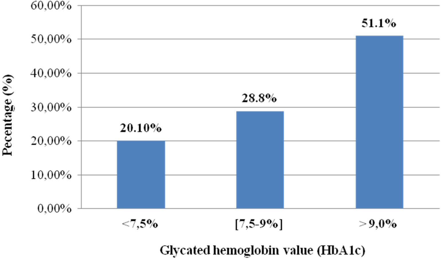
The mean age of the patients surveyed was 8.49 ± 4.1 years; the majority (68.5%) was of school age, female (53.2%) and was from low socioeconomic level (83.2%). Only 20.1% of the patients had a good glycemic control. The low socioeconomic status and overweight or obesity were significantly more prevalent in children with poor compared to those with good glycemic control (P ≤ 0.001). Multivariate analysis revealed an association of poor glycemic control with the family history of diabetes (adjusted OR = 38.70, 95% CI: 11.61, 128.98) and the absence of therapeutic education (adjusted OR = 3.29, 95% CI: 1.006, 10.801).
This study shows that diabetes is associated with overweight and obesity in children and that the quality of glycemic control is generally poor in these patients. The data showed also that improving the quality of life of T1D patients requires good therapeutic education, hence the need to introduce a real national policy.
Citation: Sanaa El–Jamal, Houda Elfane, Imane Barakat, Khadija Sahel, Mohamed Mziwira, Aziz Fassouane, Rekia Belahsen. Association of socio-demographic and anthropometric characteristics with the management and glycemic control in type 1 diabetic children from the province of El Jadida (Morocco)[J]. AIMS Medical Science, 2021, 8(2): 87-104. doi: 10.3934/medsci.2021010
Diabetes is a real public health problem in children and adolescents because of its chronicity and the difficulty in the control of blood glucose levels at paediatric age.
The aim of this study was to assess the link of socio-demographic and anthropometric characteristics with the management and glycemic control in children with type1 diabetes (T1D).
The study included a sample of 184 children with T1D of 15 years old or less. A structured questionnaire was used to collect information on socio-demographic status, characteristics and complications of the disease, diabetes management, diet, physical activity and therapeutic education of participants. Weight and height were measured and body mass index calculated.
The mean age of the patients surveyed was 8.49 ± 4.1 years; the majority (68.5%) was of school age, female (53.2%) and was from low socioeconomic level (83.2%). Only 20.1% of the patients had a good glycemic control. The low socioeconomic status and overweight or obesity were significantly more prevalent in children with poor compared to those with good glycemic control (P ≤ 0.001). Multivariate analysis revealed an association of poor glycemic control with the family history of diabetes (adjusted OR = 38.70, 95% CI: 11.61, 128.98) and the absence of therapeutic education (adjusted OR = 3.29, 95% CI: 1.006, 10.801).
This study shows that diabetes is associated with overweight and obesity in children and that the quality of glycemic control is generally poor in these patients. The data showed also that improving the quality of life of T1D patients requires good therapeutic education, hence the need to introduce a real national policy.
International Diabetes Federation
Type 1 diabetes
International Society for Paediatric and Adolescent Diabetes
Diabetes control and complications trial
Glycated haemoglobin
World Health Organization
Waist circumference
Waist-to-Height ratio
Body mass index
Standard deviations
Fasting blood glucose
Postprandial blood glucose
Odds ratio
Confidence interval
Medical assistance scheme
American Diabetes Association
Versus

| [1] | International Diabetes Federation (IDF) (2019) Diabetes in the young: a global perspective. IDF Diabetes Atlas Brussels: International Diabetes Federation, Available from: www.idf.org. |
| [2] |
The Diabetes Control and Complications Trial/Epidemiology of Diabetes Interventions and Complications Research Group (2000) Retinopathy and nephropathy in patients with type 1 diabetes four years after a trial of intensive therapy. N Engl J Med 342: 381-389. [Erratum in: |
| [3] |
DiMeglio LA, Acerini CL, Codner E, et al. (2018) ISPAD Clinical Practice Consensus Guidelines 2018: Glycemic control targets and glucose monitoring for children, adolescents, and young adults with diabetes. Pediatr Diabetes 19: 105-114. doi: 10.1111/pedi.12737

|
| [4] |
Amuna P, Zotor FB (2008) Epidemiological and nutrition transition in developing countries: impact on human health and development. Proc Nutr Soc 67: 82-90. doi: 10.1017/S0029665108006058
|
| [5] | Ministry of Health Report of the national survey on common risk factors for non communicable diseases, STEPS, Morocco (2017–2018) .Available from: https://www.who.int/ncds/surveillance/steps/STEPS-REPORT-2017-2018-Morocco-final.pdf. |
| [6] | Balafrej A (2003) Management of diabetic children at the University Hospital Center of Rabat: an example of partnership or personal initiative on the periphery of the School of Medicine? Public Health 15: 163-168. (In French). |
| [7] | Nathan DM, DCCT/EDIC Research Group (2014) The diabetes control and complications trial/epidemiology of diabetes interventions and complications study at 30 years: overview. Diabetes Care 37: 9-16. |
| [8] | Tubiana-Rufi N, Czernichow P (2003) Special problems and management of the child less than 5 years of age. Contemporary Endocrinology: Type 1 Diabetes: Etiology and Treatment New Jersey, USA: SHP Inc, 279-292. |
| [9] | American Diabetes Association (2021) Children and adolescents: standards of medical care diabetes–2021. Diabetes Care 44: S180-S199. |
| [10] |
Miller KM, Foster NC, Beck RB, et al. (2015) Current state of type 1 diabetes treatment in the U.S.: updated data from the T1D exchange clinic registry. Diabetes Care 38: 971-978. doi: 10.2337/dc15-0078
|
| [11] |
Rosenbauer J, Dost A, Karges B, et al. (2012) Improved metabolic control in children andadolescents with type 1 diabetes: a trend analysis using prospective multicenter data from Germany and Austria. Diabetes Care 35: 80-86. doi: 10.2337/dc11-0993
|
| [12] | Purnell JQ (2000) Definitions, Classification, and Epidemiology of Obesity. [Updated 2018 Apr 12]. Endotext [Internet] South Dartmouth (MA): MDText.com, Inc, Available from: https://www.ncbi.nlm.nih.gov/books/NBK279167. |
| [13] |
McCarthy HD, Ashwell M (2006) A study of central fatness using waist-to-height ratios in UK children and adolescents over two decades supports the simple message—“keep your waist circumference to less than half your height”. Int J Obes (Lond) 30: 988-992. doi: 10.1038/sj.ijo.0803226
|
| [14] | WHOAnthro (version 1.0.4, January 2011) and macros [Internet]. [cité 5 mai 2012] Available from: http://www.who.int/childgrowth/software/en/. |
| [15] | WHO Child Growth StandardsLength/height-for-age, weight-for-age, weight-for-length, weight-for-height and body mass index-for-age. Methods and development (2006) .Available from: https://www.who.int/childgrowth/standards/Technical_report.pdf?ua=1. |
| [16] | World Health Organization: WHO Child Growth Standards (2007) Growth reference data for 5–19 years Available from: http://www.who.int/growthref/en/. |
| [17] |
Butte NF, Garza C, de Onis M (2007) Evaluation of the feasibility of international growth standards for school-aged children and adolescents. J Nutr 137: 153-157. doi: 10.1093/jn/137.1.153
|
| [18] |
Rewers M, Pihoker C, Donaghue K, et al. (2007) Assessment and monitoring of glycemic control in children and adolescents with diabetes. Pediatr Diabetes 8: 408-418. doi: 10.1111/j.1399-5448.2007.00352.x
|
| [19] | International Diabetes Federation Global IDF/ISPAD guideline for diabetes in childhood and adolescence (2011) .Available from: https://cdn.ymaws.com/www.ispad.org/resource/resmgr/Docs/idf-ispad_guidelines_2011_0.pdf. |
| [20] | Karkouri FZModalities of care for diabetic children at Marrakech University Hospital. Morocco (thesis) (2017) . |
| [21] | Bensenouci A, Achir M, Boukari R, et al. (2014) Management of type 1 diabetic children in Algeria (Diab Care Pediatric). Med Metab Dis 8: 646-651. |
| [22] |
Ben Becher S, Chéour M, Essadam L, et al. (2009) Management of type 1 diabetes in childhood in Tunis: current report and perspectives. Arch Pediatr 16: 866-867. (in French). doi: 10.1016/S0929-693X(09)74183-1
|
| [23] |
Anderson BJ, Auslander WF, Jung KC, et al. (1990) Assessing family sharing of diabetes responsibilities. J Pediatr Psychol 15: 477-492. doi: 10.1093/jpepsy/15.4.477
|
| [24] |
Edwards R, Burns JA, McElduff P, et al. (2003) Variations in process and outcomes of diabetes care by socio-economic status in Salford, UK. Diabetologia 46: 750-759. doi: 10.1007/s00125-003-1102-z
|
| [25] |
Benjelloun S (2002) Nutrition transition in Morocco. Public Health Nutr 5: 135-140. doi: 10.1079/PHN2001285
|
| [26] | World Health Organization World diabetes report (2016) .Available from: https://apps.who.int/iris/bitstream/handle/10665/254648/9789242565256-fre.pdf. |
| [27] |
Belahsen R (2014) Nutrition transition and food sustainability. Proc Nutr Soc 73: 385-388. doi: 10.1017/S0029665114000135
|
| [28] |
Liu LL, Lawrence JM, Davis C, et al. (2010) Prevalence of overweight and obesity in youth with diabetes in USA: the SEARCH for Diabetes in Youth study. Pediatr Diabetes 11: 4-11. doi: 10.1111/j.1399-5448.2009.00519.x
|
| [29] |
Boucher-Berry C, Parton EA, Alemzadeh R (2016) Excess weight gain during insulin pump therapy is associated with higher basal insulin doses. J Diabetes Metab Disord 15: 47. doi: 10.1186/s40200-016-0271-5
|
| [30] |
Pinhas-Hamiel O, Levek-Motola N, Kaidar K, et al. (2015) Prevalence of overweight, obesity and metabolic syndrome components in children, adolescents and young adults with type 1 diabetes mellitus. Diabetes Metab Res Rev 31: 76-84. doi: 10.1002/dmrr.2565
|
| [31] |
Minges KE, Whittemore R, Weinzimer SA, et al. (2017) Correlates of overweight and obesity in 5,529 adolescents with type 1 diabetes: the T1D exchange clinic registry. Diabetes Res Clin Pract 126: 68-78. doi: 10.1016/j.diabres.2017.01.012
|
| [32] |
Hogel J, Grabert M, Sorgo W, et al. (2000) Hemoglobin A1c and body mass index in children and adolescents with IDDM. An observational study from 1976–1995. Exp Clin Endocrinol Diabetes 108: 76-80. doi: 10.1055/s-2000-5799
|
| [33] |
Huppertz E, Pieper L, Klotsche J, et al. (2009) Diabetes mellitus in German primary care: quality of glycaemic control and subpopulations not well controlled-results of the DETECT study. Exp Clin Endocrinol Diabetes 117: 6-14. doi: 10.1055/s-2008-1073127
|
| [34] |
Hughes CR, McDowell N, Cody D, et al. (2012) Sustained benefits of continuous subcutaneous insulin infusion. Arch Dis Child 97: 245-247. doi: 10.1136/adc.2010.186080
|
| [35] |
Nathan DM, Cleary PA, Backlund JY, et al. (2005) Intensive diabetes treatment and cardiovascular disease in patients with type 1 diabetes. N Engl J Med 353: 2643-2653. doi: 10.1056/NEJMoa052187
|
| [36] |
Rosenbauer J, Dost A, Karges B, et al. (2012) The DPV Initiative and the German BMBF Competence Network Diabetes Mellitus. Improved metabolic control in children and adolescents with type 1 diabetes: a trend analysis using prospective multicenter data from Germany and Austria. Diabetes Care 35: 80-86. doi: 10.2337/dc11-0993
|
| [37] |
Nordly S, Mortensen HB, Andreasen AH, et al. (2005) Factors associated with glycaemic outcome of childhood diabetes care in Denmark. Diabet Med 22: 1566-1573. doi: 10.1111/j.1464-5491.2005.01692.x
|
| [38] | Guilmin-Crépon S, Tubiana-Rufi N (2010) Self-monitoring of blood glucose in children and adolescent with type 1 diabetes. Med Metab Dis 4: S12-S19. |
| [39] |
Asvold BO, Sand T, Hestad K, et al. (2010) Cognitive function in type 1 diabetic adults with early exposure to severe hypoglycemia: a 16-year follow-up study. Diabetes Care 33: 1945-1947. doi: 10.2337/dc10-0621
|
| [40] |
Hanas R, Lindgren F, Lindblad B (2009) A 2-year national population study of pediatric ketoacidosis in Sweden: predisposing conditions and insulin pump use. Pediatr Diabetes 10: 33-37. doi: 10.1111/j.1399-5448.2008.00441.x
|
| [41] |
Nordwall M, Arnqvist HJ, Bojestig M, et al. (2009) Good glycemic control remains crucial in prevention of late diabetic complications—the Linkoping Diabetes Complications Study. Pediatr Diabetes 10: 168-176. doi: 10.1111/j.1399-5448.2008.00472.x
|
| [42] |
Lièvre M, Marre M, Robert JJ, et al. (2005) Cross-sectional study of care, socio-economic status and complications in young French patients with type 1 diabetes mellitus. Diabetes Metab 31: 41-46. doi: 10.1016/S1262-3636(07)70165-9
|
| [43] |
Katamay SW, Esslinger KA, Vigneault M, et al. (2007) Eating well with Canada's Food Guide (2007): development of the food intake pattern. Nutr Rev 65: 155-166. doi: 10.1301/nr.2007.apr.155-166
|
| [44] |
Patrick K, Norman GJ, Calfas KJ, et al. (2004) Diet, physical activity and sedentary behaviors as risk factors for overweight in adolescence. Arch Pediatr Adolesc Med 158: 385-390. doi: 10.1001/archpedi.158.4.385
|
| [45] |
Michaliszyn FS, Shaibi GQ, Quinn L, et al. (2009) Physical fitness, dietary intake, and metabolic control in adolescents with type 1 diabetes. Pediatr Diabetes 10: 389-394. doi: 10.1111/j.1399-5448.2009.00500.x
|
| [46] |
Mayer-Davis EJ, Nichols M, Liese AD, et al. (2006) Dietary intake among youth with diabetes: the SEARCH for diabetes in youth study. J Am Diet Assoc 106: 689-697. doi: 10.1016/j.jada.2006.02.002
|
| [47] |
Riddell MC, Gallen IW, Smart CE, et al. (2017) Exercise management in type 1 diabetes: a consensus statement. Lancet Diabetes Endocrinol 5: 377-390. doi: 10.1016/S2213-8587(17)30014-1
|
| [48] |
Warburton DER, Nicol CW, Bredin SSD (2006) Health benefits of physical activity: the evidence. CMAJ 174: 801-809. doi: 10.1503/cmaj.051351
|
| [49] |
Quirk H, Blake H, Tennyson R, et al. (2014) Physical activity interventions in children and young people with type 1 diabetes mellitus: a systematic review with meta-analysis. Diabet Med 31: 1163-1173. doi: 10.1111/dme.12531
|
| [50] |
Kummer S, Stahl-Pehe A, Castillo K, et al. (2014) Health behaviour in children and adolescents with type 1 diabetes compared to a representative reference population. PLoS One 9: e112083. doi: 10.1371/journal.pone.0112083
|
| [51] |
Chimen M, Kennedy A, Nirantharakumar K, et al. (2012) What are the health benefits of physical activity in type 1 diabetes mellitus? A literature review. Diabetologia 55: 542-551. doi: 10.1007/s00125-011-2403-2
|
| [52] |
Guerci B, Tubiana-Rufi N, Bauduceau B, et al. (2005) Advantages to using capillary blood β–hydroxybutyrate determination for the detection and treatment of diabetic ketosis. Diabetes Metab 31: 401-406. doi: 10.1016/S1262-3636(07)70211-2
|
| [53] |
Von Sengbusch S, Muller-Godeffroy E, Hager S, et al. (2006) Mobile diabetes education and care: intervention for children and young people with Type 1 diabetes in rural areas of northern Germany. Diabet Med 23: 122-127. doi: 10.1111/j.1464-5491.2005.01754.x
|
| [54] |
Swift PGF, Skinner TC, De Beaufort CE, et al. (2010) Target setting in intensive insulin management is associated with metabolic control: the Hvidoere childhood diabetes study group centre differences study 2005. Pediatr Diabetes 11: 271-278. doi: 10.1111/j.1399-5448.2009.00596.x
|
| [55] |
Mortensen HB, Robertson KJ, Aanstoot HJ, et al. (1998) Insulin management and metabolic control of Type 1 Diabetes Mellitus in Childhood and Adolescence in 18 Countries. Hvidøre Study Group on Childhood Diabetes. Diabet Med 15: 752-759. doi: 10.1002/(SICI)1096-9136(199809)15:9<752::AID-DIA678>3.0.CO;2-W
|
| [56] | The Diabetes Control and Complications Trial Research Group (1993) The effect of intensive treatment of diabetes on the development and progression of long-term complications in insulin- dependent diabetes mellitus. N Engl J Med 329: 977-986. |
| [57] | Geoffroy L, Gonthier M (2012) Diabetes in children and adolescents Montreal: Ste-Justine University Hospital Center, 451-465. |
| [58] | Tfayli H, Arslanian S The challenge of adolescence: Hormonal changes and insulin sensitivity [Online] (2007) .Available from: https://studylibfr.com/doc/3271994/le-d%C3%A9fi-de-l-adolescence---changements-hormonaux-et-sensi. |
Figures(1) / Tables(4)

Sanaa El–Jamal, Houda Elfane, Imane Barakat, Khadija Sahel, Mohamed Mziwira, Aziz Fassouane, Rekia Belahsen. Association of socio-demographic and anthropometric characteristics with the management and glycemic control in type 1 diabetic children from the province of El Jadida (Morocco)[J]. AIMS Medical Science, 2021, 8(2): 87-104. doi: 10.3934/medsci.2021010


 DownLoad: