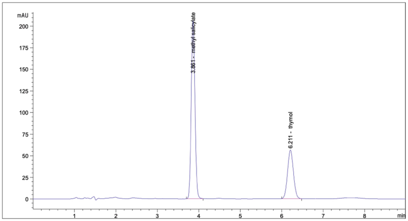
Various topical formulations comprise of methyl salicylate and thymol due to their analgesic and anti-inflammatory properties. The huge demand has led traditional medicines being susceptible to adulteration with synthetic drugs or their analogues to enhance their efficacy and to minimise the cost of obtaining the limited natural substance. The objectives of this study are to analyse a suitable analytical method for simultaneous determination of methyl salicylate and thymol in selected Malaysian traditional medicines using High Performance Liquid Chromatography (HPLC) and to screen the selected Malaysian traditional medicines for possible methyl salicylate and thymol adulteration using the analytical method. Most literature search showed the determination of methyl salicylate and thymol as an individual compound or in combination with other compounds instead of both being detected simultaneously using a single method. Methyl salicylate and thymol were separated at about 3.8 and 6.2 min, respectively at a flow rate of 1 mL/min on C8 column with methanol and water (65: 35) as the mobile phase, column temperature of 35 °C and detector wavelength of 230 nm within 9 minutes of run time. Method validation was conducted and this method was sensitive, linear, specific, precise and accurate. The validated method was applied for screening of methyl salicylate and thymol in 10 samples of liniment and ointment. Half of the samples were detected with methyl salicylate and none with thymol. Majority of the positive samples were unregistered traditional medicines. As quantitation of both compounds is achievable with this method, it will be beneficial in the regulatory and industrial settings. This will ensure the safety and quality of traditional medicines, thereby safeguarding consumer's health. Hence, the method can be adopted for routine quality control (QC) analysis of methyl salicylate and thymol in traditional medicines.
Citation: Muhammad Shahariz Mohamad Adzib, Zul Ilham. Simultaneous analytical determination of methyl salicylate and thymol in selected Malaysian traditional medicines[J]. AIMS Medical Science, 2020, 7(2): 43-56. doi: 10.3934/medsci.2020004
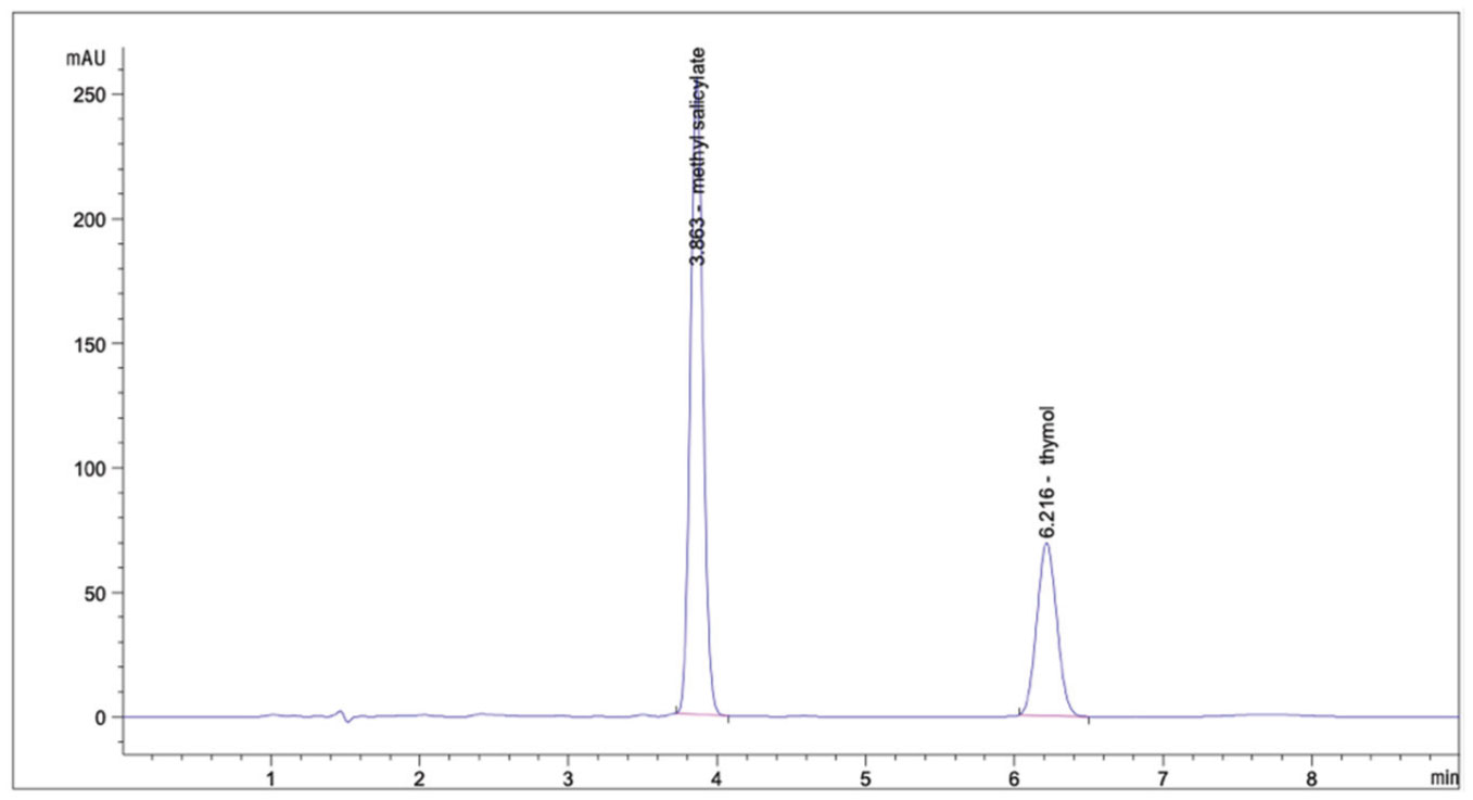
Various topical formulations comprise of methyl salicylate and thymol due to their analgesic and anti-inflammatory properties. The huge demand has led traditional medicines being susceptible to adulteration with synthetic drugs or their analogues to enhance their efficacy and to minimise the cost of obtaining the limited natural substance. The objectives of this study are to analyse a suitable analytical method for simultaneous determination of methyl salicylate and thymol in selected Malaysian traditional medicines using High Performance Liquid Chromatography (HPLC) and to screen the selected Malaysian traditional medicines for possible methyl salicylate and thymol adulteration using the analytical method. Most literature search showed the determination of methyl salicylate and thymol as an individual compound or in combination with other compounds instead of both being detected simultaneously using a single method. Methyl salicylate and thymol were separated at about 3.8 and 6.2 min, respectively at a flow rate of 1 mL/min on C8 column with methanol and water (65: 35) as the mobile phase, column temperature of 35 °C and detector wavelength of 230 nm within 9 minutes of run time. Method validation was conducted and this method was sensitive, linear, specific, precise and accurate. The validated method was applied for screening of methyl salicylate and thymol in 10 samples of liniment and ointment. Half of the samples were detected with methyl salicylate and none with thymol. Majority of the positive samples were unregistered traditional medicines. As quantitation of both compounds is achievable with this method, it will be beneficial in the regulatory and industrial settings. This will ensure the safety and quality of traditional medicines, thereby safeguarding consumer's health. Hence, the method can be adopted for routine quality control (QC) analysis of methyl salicylate and thymol in traditional medicines.

| [1] | Anderson A, Mcconville A, Fanthorpe L, et al. (2017) Salicylate poisoning potential of topical pain relief agents: from age old remedies to engineered smart patches. Medicines 4: 1-13. |
| [2] | Bachute MT, Shanbhag SV (2016) Analytical method development for simultaneous estimation of methyl salicylate, methol, thymol and camphor in an ointment and its validation by Gas Chromatography. Int J Chem Pharm Anal 3: 1-11. |
| [3] | Nagoor Meeran MF, Javed H, Taee HA, et al. (2017) Pharmacological properties and molecular mechanisms of thymol: Prospects for its therapeutic potential and pharmaceutical development. Front Pharmacol 8: 1-34. |
| [4] | Abubakar BM, Salleh FM, Omar MS, et al. (2018) Assessing product adulteration of Eurycoma longifolia (Tongkat Ali) herbal medicinal product using DNA barcoding and HPLC analysis. Pharm Biol 56: 1-10. |
| [5] | Haneef J, Shaharyar M, Husain A, et al. (2013) Analytical methods for the detection of undeclared synthetic drugs in traditional herbal medicines as adulterants. Drug Test Anal 5: 607-613. |
| [6] | (2005) International Council for Harmonisation of Technical Requirements for Pharmaceuticals for Human Use, ICH Topic Q2 (R1) Validation of Analytical Procedures: Text and Methodology. International Council for Harmonisation of Technical Requirements for Pharmaceuticals for Human Use Available from: https://database.ich.org/sites/default/files/Q2_R1__Guideline.pdf. |
| [7] | Shabir GA (2005) Step-by-Step analytical methods validation and protocol in the quality system compliance industry. J Valid Technol 10: 314-324. |
| [8] | Shabir GA, Lough WJ, Arain SA, et al. (2007) Evaluation and application of best practice in analytical method validation. J Liq Chromatogr Relat Technol 30: 311-333. |
| [9] | Shabir GA, Bradshaw TK (2011) Development and validation of a Liquid Chromatography method for the determination of methyl salicylate in a medicated cream formulation. Turk J Pharm Sci 8: 117-126. |
| [10] | (2013) AOAC International, AOAC Guidelines for Single Laboratory Validation of Chemical Methods for Dietary Supplements and Botanicals. AOAC International Available from: http://members.aoac.org/aoac_prod_imis/AOAC_Docs/StandardsDevelopment/SLV_Guidelines_Dietary_Supplements.pdf. |
| [11] | (2017) MyHEALTH, Adulteration in Traditional Medicine Products. Ministry of Health MY Available from: http://www.myhealth.gov.my/en/adulteration-traditional-medicine-products/. |
| [12] | Posadzki P, Watson L, Ernst E (2012) Contamination and adulteration of herbal medicinal products (HMPs): An overview of systematic reviews. Eur J Clin Pharmacol 69: 295-307. |
| [13] | (2019) National Pharmaceutical Regulatory Agency, Cancellation of Registered Complementary and Alternative Product. National Pharmaceutical Regulatory Agency Available from: https://www.npra.gov.my/index.php/en/consumers/safety-information/cancellation-of-registered-complementary-alternative-product.html. |
| [14] | (2016) National Pharmaceutical Regulatory Division, Drug Registration Guidance Document (DRGD). National Pharmaceutical Regulatory Division Available from: https://www.npra.gov.my/index.php/en/drug-registration-guidance-documents-drgd-e-book.html. |
| [15] | Zakaria M, Vijayasekaran, Ilham Z, et al. (2014) Anti inflammatory activity of Calophyllum inophyllum fruit extracts. Procedia Chem 13: 218-220. |
| [16] | Chang X, Sun P, Ma Y, et al. (2020) A new method for determination of thymol and carvacrol in Thymi herba by Ultraperformance Convergence Chromatography (UPC2). Molecules 25: 1-11. |
 medsci-07-02-004-s01.pdf medsci-07-02-004-s01.pdf |
 |

Figures(6) / Tables(3)

Muhammad Shahariz Mohamad Adzib, Zul Ilham. Simultaneous analytical determination of methyl salicylate and thymol in selected Malaysian traditional medicines[J]. AIMS Medical Science, 2020, 7(2): 43-56. doi: 10.3934/medsci.2020004


 DownLoad: