Application of <sup>212</sup>Pb for Targeted α-particle Therapy (TAT): Pre-clinical and Mechanistic Understanding through to Clinical Translation

Kwon Yong; Martin Brechbiel; Kwon Yong; Martin Brechbiel

doi:10.3934/medsci.2015.3.228

AIMS Medical Science

2015, Volume 2, Issue 3: 228-245. doi: 10.3934/medsci.2015.3.228

Previous Article Next Article

Review

Application of ²¹²Pb for Targeted α-particle Therapy (TAT): Pre-clinical and Mechanistic Understanding through to Clinical Translation

Kwon Yong ,
Martin Brechbiel ^,

Radioimmune & Inorganic Chemistry Section, Radiation Oncology Branch, National Cancer Institute, National Institutes of Health, Bethesda MD, USA

Received: 20 April 2015 Accepted: 12 August 2015 Published: 18 August 2015

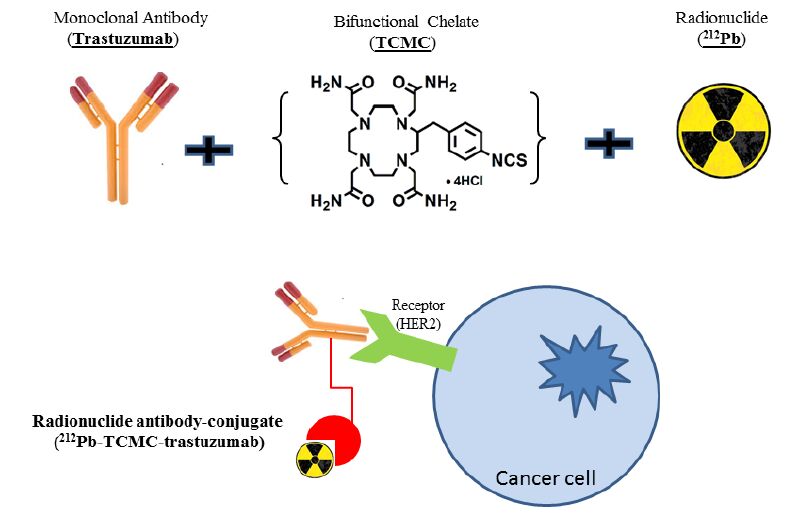
Targeted α-particle therapy (TAT), in which an α-particle emitting radionuclide is specifically directed to a biological target, is gaining more attention to treat cancers as new targets are validated. Bio-vectors such as monoclonal antibodies are able to selectively transport α-particles to destroy targeted cancer cells. TAT has the potential for an improved therapeutic ratio over β-particle targeted conjugate therapy. The short path length and the intense ionization path generated render α-emitters suitable for treatment and management of minimal disease such as micrometastases or residual tumor after surgical debulking. ²¹²Pb is the longer-lived parent radionuclide of ²¹²Bi and serves as an in vivo generator of ²¹²Bi. ²¹²Pb has demonstrated significant utility in both in vitro and in vivo models. Recent evaluation of ²¹²Pb-TCMC-trastuzumab in a Phase I clinical trial has demonstrated the feasibility of ²¹²Pb in TAT for the treatment of ovarian cancer patients. This review highlights progress in radionuclide production, radiolabeling chemistry, molecular mechanisms, and application of ²¹²Pb to targeted pre-clinical and clinical radiation therapy for the management and treatment of cancer.

Keywords:

Citation: Kwon Yong, Martin Brechbiel. Application of 212Pb for Targeted α-particle Therapy (TAT): Pre-clinical and Mechanistic Understanding through to Clinical Translation[J]. AIMS Medical Science, 2015, 2(3): 228-245. doi: 10.3934/medsci.2015.3.228

Related Papers:

[1]	Xin Jin, Ruoli Tang, Tingzhe Pan, Xin Li, Zongyi Wang, Chao Jiang, Rui Zhang . Optimal operation of flexible IES based on energy hub and demand-side response. AIMS Energy, 2025, 13(3): 569-589. doi: 10.3934/energy.2025022
[2]	Badr Ouhammou, Fatima Zohra Gargab, Samir El idrissi kaitouni, Slimane Smouh, Rachid El mrabet, Mohammed Aggour, Abdelmajid Jamil, Tarik Kousksou . Energy saving potential diagnosis for Moroccan university campuses. AIMS Energy, 2023, 11(3): 576-611. doi: 10.3934/energy.2023030
[3]	Mohamed G Moh Almihat, MTE Kahn . Centralized control system for islanded minigrid. AIMS Energy, 2023, 11(4): 663-682. doi: 10.3934/energy.2023033
[4]	Panagiotis Fragkos . Analysing the systemic implications of energy efficiency and circular economy strategies in the decarbonisation context. AIMS Energy, 2022, 10(2): 191-218. doi: 10.3934/energy.2022011
[5]	Jin H. Jo, Jamie Cross, Zachary Rose, Evan Daebel, Andrew Verderber, David G. Loomis . Financing options and economic impact: distributed generation using solar photovoltaic systems in Normal, Illinois. AIMS Energy, 2016, 4(3): 504-516. doi: 10.3934/energy.2016.3.504
[6]	Tiansong Cui, Yanzhi Wang, Shahin Nazarian, Massoud Pedram . Profit maximization algorithms for utility companies in an oligopolistic energy market with dynamic prices and intelligent users. AIMS Energy, 2016, 4(1): 119-135. doi: 10.3934/energy.2016.1.119
[7]	Gustavo Henrique Romeu da Silva, Andreas Nascimento, Christoph Daniel Baum, Nazem Nascimento, Mauro Hugo Mathias, Mohd Amro . Renewable energy perspectives: Brazilian case study on green hydrogen production. AIMS Energy, 2025, 13(2): 449-470. doi: 10.3934/energy.2025017
[8]	Feng Tian . A wind power prediction model with meteorological time delay and power characteristic. AIMS Energy, 2025, 13(3): 517-539. doi: 10.3934/energy.2025020
[9]	Akash Talwariya, Pushpendra Singh, Mohan Lal Kolhe, Jalpa H. Jobanputra . Fuzzy logic controller and game theory based distributed energy resources allocation. AIMS Energy, 2020, 8(3): 474-492. doi: 10.3934/energy.2020.3.474
[10]	Jiashen Teh, Ching-Ming Lai, Yu-Huei Cheng . Composite reliability evaluation for transmission network planning. AIMS Energy, 2018, 6(1): 170-186. doi: 10.3934/energy.2018.1.170

Abstract

1. Introduction

A piezoelectric-type tensor is a third-order tensor, which plays an important role in physics ^{[1,2,3,4,5,6]} and engineering ^{[7,8,9,10,11]}. In particular, the largest C-eigenvalue of a piezoelectric tensor and its associated left and right C-eigenvectors play an important role in the piezoelectric effect and the converse piezoelectric effect in the solid crystal ^[12,13]. Moreover, in the process of manufacturing and developing micro/nano-electromechanical devices, the development of new multifunctional intelligent structures needs consideration piezoelectric effect ^[14,15]. In order to explore more information about piezoelectric-type tensors, Chen et al. ^[12] introduced piezoelectric-type tensors and their C-eigentriples.

Definition 1.1. [12,Definition 2.1] Let $ \mathcal{A} = (a_{ijk})\in\mathbb{R}^{n\times n\times n} $ be a third-order $ n $-dimensional tensor. If the latter two indices of $ \mathcal{A} $ are symmetric, i.e., $ a_{ijk} = a_{ikj} $, where $ i, j, k\in[n]: = \{1, 2, \ldots, n\} $, then $ \mathcal{A} $ is called a piezoelectric-type tensor. When $ n = 3 $, $ \mathcal{A} $ is called a piezoelectric tensor.

Definition 1.2. [12,Definition 2.2] Let $ \mathcal{A} = (a_{ijk})\in\mathbb{R}^{n\times n\times n} $ be a piezoelectric-type tensor. If there is a real number $ \lambda\in\mathbb{R} $, two vectors $ x: = (x_{1}, x_{2}, \ldots, x_{n})^{\top}\in\mathbb{R}^{n}\backslash\{0\} $ and $ y: = (y_{1}, y_{2}, \ldots, y_{n})^{\top}\in\mathbb{R}^{n}\backslash\{0\} $ such that

$ \left\{ {

$\begin{array}{*{20}{l}} {{\cal A}yy = \lambda x, }&&&&&{(1.1)}\\ {x{\cal A}y = \lambda y, }&&&&&{(1.2)}\\ {{x^ \top }x = 1, }&&&&&{(1.3)}\\ {{y^ \top }y = 1, }&&&&&{(1.4)} \end{array}$ } \right. $

where

$\begin{eqnarray*} (\mathcal{A}yy)_{i}: = \sum\limits_{j, k\in[n]}a_{ijk}y_{j}y_{k}, \quad (x\mathcal{A}y)_{k}: = \sum\limits_{i, j\in[n]}a_{ijk}x_{i}y_{j}, \end{eqnarray*}$ $

then $ \lambda $ is called a C-eigenvalue of $ \mathcal{A} $, and $ x $ and $ y $ are its associated left and right C-eigenvectors, respectively. Then, $ (\lambda, x, y) $ is called a C-eigentriple of $ \mathcal{A} $ and $ \sigma(\mathcal{A}) $ is used to denote the spectrum of $ \mathcal{A} $, which is a set of all C-eigenvalues of $ \mathcal{A} $.

Chen et al. provided the following results for the C-eigenvalues and C-eigenvectors of a piezoelectric-type tensor.

Property 1.1. [12,Theorem 2.3] Let $ \mathcal{A} = (a_{ijk})\in\mathbb{R}^{n\times n\times n} $ be a piezoelectric-type tensor.

(a) The C-eigenvalues of $ \mathcal{A} $ and their associated left and right C-eigenvectors always exist.

(b) Let $ \lambda $ be a C-eigenvalue and $ (x, y) $ be its associated left and right C-eigenvectors. Then

$\begin{eqnarray*} \lambda = x\mathcal{A}yy: = \sum\limits_{i, j, k\in[n]}a_{ijk}x_{i}y_{j}y_{k}. \end{eqnarray*}$ $

Furthermore, $ (\lambda, x, -y) $, $ (-\lambda, -x, y) $ and $ (-\lambda, -x, -y) $ are also C-eigentriples of $ \mathcal{A} $.

(c) Let $ \lambda^{*} $ be the largest C-eigenvalue of $ \mathcal{A} $. Then

$\begin{eqnarray*} \lambda^{*} = \max\{x\mathcal{A}yy:x^{\top}x = 1, y^{\top}y = 1\}. \end{eqnarray*}$ $

As we all know, the largest C-eigenvalue of a piezoelectric-type tensor and its associated C-eigenvectors constitute the best rank-one piezoelectric-type approximation. In view of this, Liang and Yang ^[16,17] designed two methods to calculate the largest C-eigenvalue of a piezoelectric-type tensor. Later, Zhao and Luo ^[18] provided a method to calculate all C-eigentriples of a piezoelectric-type tensor by converting the C-eigenvalue problem to the Z-eigenvalue problem of tensors. Moreover, many researchers considered the C-eigenvalue localization problem and provided many C-eigenvalue localization sets ^{[19,20,21,22,23,24]}. For instance, Che et al. ^[25] presented the following Geršgorin-type C-eigenvalue localization set.

Theorem 1.1. [25,Theorem 2.1] Let $ \mathcal{A} = (a_{ijk})\in\mathbb{R}^{n\times n\times n} $ be a piezoelectric-type tensor. Then

$\begin{eqnarray*} \sigma(\mathcal{A})\subseteq\Gamma(\mathcal{A}): = \bigcup\limits_{j\in[n]}\Gamma_j(\mathcal{A}), \end{eqnarray*}$ $

where

$\begin{eqnarray*} \Gamma_j(\mathcal{A}): = \{z\in\mathbb{R}: |z|\leq R_j(\mathcal{A})\} \quad\mathit{{and}}\quad R_j(\mathcal{A}): = \sum\limits_{l, k\in[n]}|a_{lkj}|. \end{eqnarray*}$ $

Definition 1.2 and Property 1.1 indicate that a C-eigenvalue $ \lambda $ is real and both $ \lambda $ and $ -\lambda $ are C-eigenvalues, which implies that a C-eigenvalue localization set is always symmetric with respect to the origin. Therefore, the result of Theorem 1.1 is equivalent to $ \sigma(\mathcal{A})\subseteq[-\rho_\Gamma, \rho_\Gamma] $, where $ \rho_\Gamma = \max\limits_{j\in[n]}\{R_j(\mathcal{A})\} $.

The remainder of the paper is organized as follows. In Section 2, we construct a new C-eigenvalue localization set and prove that it is sharper than some existing sets. In Section 3, we provide a direct method to find all C-eigentriples when $ n = 3 $. In Section 4, we reviewed the practical application of C-eigentriples of a piezoelectric-type tensor to the piezoelectric effect and converse piezoelectric effect. In Section 5, we verify the effectiveness of obtained results by numerical examples. In Section 6, we give a summary of this paper.

2. A new C-eigenvalue localization set

In this section, we provide a new C-eigenvalue localization set and prove that it is sharper than the set in Theorem 1.1. Before that, the following lemma is needed.

Lemma 2.1. [26,pp. 10, Cauchy-Schwarz inequality] Let $ x = (x_1, x_2, \ldots, x_n)^{\top}\in\mathbb{R}^{n} $ and $ y = (y_1, y_2, \ldots, y_n)^{\top}\in\mathbb{R}^{n} $. Then

$\begin{eqnarray*} \Big(\sum\limits_{i\in[n]}x_{i}y_{i}\Big)^{2}\leq\sum\limits_{i\in[n]}x_{i}^2\sum\limits_{i\in[n]}y_{i}^2. \end{eqnarray*}$ $

Theorem 2.1. Let $ \mathcal{A} = (a_{ijk})\in\mathbb{R}^{n\times n\times n} $ be a piezoelectric-type tensor. Then

$\begin{eqnarray*} \sigma(\mathcal{A})\subseteq\Omega(\mathcal{A}): = \Bigg(\bigcup\limits_{i\in[n]}\widehat{\Omega}_{i}(\mathcal{A})\Bigg)\cup\Bigg(\bigcup\limits_{i, j\in[n], i\neq j} \Big(\widetilde{\Omega}_{i, j}(\mathcal{A})\cap\mathcal{K}_{i}(\mathcal{A})\Big)\Bigg), \end{eqnarray*}$ $

where

$\begin{align*} \widehat{\Omega}_{i}(\mathcal{A})&: = \{z\in\mathbb{R}: |z|\leq \overline{r}_{i}^i(\mathcal{A})\}, \\ \widetilde{\Omega}_{i, j}(\mathcal{A})&: = \{z\in\mathbb{R}: (|z|-\overline{r}_{i}^i(\mathcal{A}))(|z|-\widetilde{r}_{j}^i(\mathcal{A}))\leq\widetilde{r}_{i}^i(\mathcal{A})\overline{r}_{j}^i(\mathcal{A})\}, \\ \mathcal{K}_{i}(\mathcal{A})&: = \{z\in\mathbb{R}: |z|\leq r_{i}(\mathcal{A})\}, \end{align*}$ $

and

$\begin{align*} &\overline{r}_j^{i}(\mathcal{A}): = \sqrt{\sum\limits_{l\in[n]}a_{lij}^2}, \quad \widetilde{r}_j^i(\mathcal{A}): = \sqrt{\sum\limits_{l\in[n]}\Big(\sum\limits_{k\in[n], k\neq i}|a_{lkj}|\Big)^2}, \\ &r_i(\mathcal{A}): = \sqrt{\sum\limits_{l\in[n]}\Big(\sum\limits_{k\in[n]}|a_{lki}|\Big)^2}, \quad i, j\in [n]. \end{align*}$ $

Proof. Let $ (\lambda, x, y) $ be a C-eigentriple of $ \mathcal{A} $. Let $ |y_{t}|\geq |y_{s}| \geq \max\limits_{k\in [n], k\neq t, k\neq s} \{|y_{k}|\} $. Then $ 0\leq |y_{t}|\leq 1 $. From (1.2), we have

$\begin{eqnarray*} \lambda y_{t} = \sum\limits_{l, k\in[n]}a_{lkt}x_{l}y_{k} = \sum\limits_{l\in[n]}a_{ltt}x_{l}y_{t}+\sum\limits_{l, k\in[n], k\neq t}a_{lkt}x_{l}y_{k}. \end{eqnarray*}$ $

Taking the modulus in above equation and using the triangle inequality and Lemma 2.1, we have

$\begin{align*} |\lambda||y_t|& \leq\sum\limits_{l, k\in[n]}|a_{lkt}||x_{l}||y_t| = |y_t|\sum\limits_{l\in[n]}\Big(|x_{l}|\sum\limits_{k\in[n]}|a_{lkt}|\Big)\\ &\leq|y_t|\sqrt{\sum\limits_{l\in[n]}|x_{l}|^2}\sqrt{\sum\limits_{l\in[n]}\Big(\sum\limits_{k\in[n]}|a_{lkt}|\Big)^2} = |y_t|\sqrt{\sum\limits_{l\in [n]}\Big(\sum\limits_{k\in[n]}|a_{lkt}|\Big)^2}, \end{align*}$ $

i.e.,

$\begin{eqnarray*} |\lambda|\leq \sqrt{\sum\limits_{l\in[n]}\Big(\sum\limits_{k\in[n]}|a_{lkt}|\Big)^2} = r_t(\mathcal{A}), \end{eqnarray*}$ $

which implies that $ \lambda\in\mathcal{K}_t(\mathcal{A}) $, and

$\begin{align*} |\lambda||y_{t}|&\leq\sum\limits_{l\in[n]}|a_{ltt}||x_{l}||y_{t}|+\sum\limits_{l, k\in[n], k\neq t}|a_{lkt}||x_{l}||y_{k}|\\ &\leq\sum\limits_{l\in[n]}|a_{ltt}||x_{l}||y_{t}|+\sum\limits_{l, k\in[n], k\neq t}|a_{lkt}||x_{l}||y_{s}|\\ & = |y_{t}|\sum\limits_{l\in[n]}|a_{ltt}||x_{l}|+|y_{s}|\sum\limits_{l\in[n]}\Big(|x_{l}|\sum\limits_{k\in[n], k\neq t}|a_{lkt}|\Big)\\ &\leq|y_{t}|\sqrt{\sum\limits_{l\in[n]}a_{ltt}^2}\sqrt{\sum\limits_{l\in[n]}x_l^2} +|y_s|\sqrt{\sum\limits_{l\in[n]}x_l^2}\sqrt{\sum\limits_{l\in [n]}\Big(\sum\limits_{k\in[n], k\neq t}|a_{lkt}|\Big)^2}\\ & = |y_{t}|\sqrt{\sum\limits_{l\in[n]}a_{ltt}^2}+|y_{s}|\sqrt{\sum\limits_{l\in[n]}\Big(\sum\limits_{k\in[n], k\neq t}|a_{lkt}|\Big)^2}\\ & = \overline{r}_{t}^t(\mathcal{A})|y_{t}|+\widetilde{r}_{t}^t(\mathcal{A})|y_{s}|, \end{align*}$ $

i.e.,

$\begin{eqnarray} (|\lambda|-\overline{r}_{t}^t(\mathcal{A}))|y_{t}|\leq\widetilde{r}_{t}^t(\mathcal{A})|y_{s}|. \end{eqnarray}$ $

(2.1)

If $ |y_{s}| = 0 $ in (2.1), we have $ |\lambda|\leq \overline{r}_{t}^t(\mathcal{A}) $, which implies that $ \lambda\in\widehat{\Omega}_{t}(\mathcal{A})\subseteq\Omega(\mathcal{A}) $.

If $ |y_{s}| > 0 $ in (2.1), then $ |\lambda|\leq \overline{r}_{t}^t(\mathcal{A})+\widetilde{r}_{t}^t(\mathcal{A})\leq r_t(\mathcal{A}) $, which implies that $ \lambda\in\mathcal{K}_{t}(\mathcal{A}) $. Now, suppose that $ \lambda\notin\widehat{\Omega}_{t}(\mathcal{A}) $, i.e., $ |\lambda| > \overline{r}_{t}^t(\mathcal{A}) $. The $ s $-th equation of (1.2) is

$\begin{eqnarray*} \lambda y_{s} = \sum\limits_{l, k\in[n]}a_{lks}x_{l}y_{k} = \sum\limits_{l\in[n]}a_{lts}x_{l}y_{t}+\sum\limits_{l, k\in[n], k\neq t}a_{lks}x_{l}y_{k}, \end{eqnarray*}$ $

which implies that

$\begin{align*} |\lambda||y_{s}|&\leq\sum\limits_{l\in[n]}|a_{lts}||x_{l}||y_{t}|+\sum\limits_{l, k\in[n], k\neq t}|a_{lks}||x_{l}||y_{k}|\\ &\leq\sum\limits_{l\in[n]}|a_{lts}||x_{l}||y_{t}|+\sum\limits_{l, k\in[n], k\neq t}|a_{lks}||x_{l}||y_{s}|\\ & = |y_{t}|\sum\limits_{l\in[n]}|a_{lts}||x_{l}|+|y_{s}|\sum\limits_{l\in[n]}\Big(|x_{l}|\sum\limits_{k\in[n], k\neq t}|a_{lks}|\Big)\\ &\leq|y_{t}|\sqrt{\sum\limits_{l\in[n]}a_{lts}^2}\sqrt{\sum\limits_{l\in[n]}x_l^2} +|y_{s}|\sqrt{\sum\limits_{l\in[n]}x_l^2}\sqrt{\sum\limits_{l\in[n]}\Big(\sum\limits_{k\in[n], k\neq t}|a_{lks}|\Big)^2}\\ & = |y_{t}|\sqrt{\sum\limits_{l\in[n]}a_{lts}^2}+|y_{s}|\sqrt{\sum\limits_{l\in[n]}\Big(\sum\limits_{k\in[n], k\neq t}|a_{lks}|\Big)^2}\\ & = \overline{r}_{s}^t(\mathcal{A})|y_{t}|+\widetilde{r}_{s}^t(\mathcal{A})|y_{s}|, \end{align*}$ $

i.e.,

$\begin{eqnarray} (|\lambda|-\widetilde{r}_{s}^t(\mathcal{A}))|y_{s}|\leq\overline{r}_{s}^t(\mathcal{A})|y_{t}|. \end{eqnarray}$ $

(2.2)

By multiplying (2.1) and (2.2) and eliminating $ |y_{s}||y_{t}| > 0 $, we have

$\begin{eqnarray*} (|\lambda|-\overline{r}_{t}^t(\mathcal{A}))(|\lambda|-\widetilde{r}_{s}^t(\mathcal{A}))\leq\widetilde{r}_{t}^t(\mathcal{A})\overline{r}_{s}^t(\mathcal{A}), \end{eqnarray*}$ $

which implies that $ \lambda\in\Big(\widetilde{\Omega}_{t, s}(\mathcal{A})\cap\mathcal{K}_{t}(\mathcal{A})\Big)\subseteq\Omega(\mathcal{A}) $, and consequently, $ \sigma(\mathcal{A})\subseteq \Omega(\mathcal{A}) $ by the arbitrariness of $ \lambda $.

Next, we discuss the relationship between the set $ \Omega(\mathcal{A}) $ in Theorem 2.1 and the set $ \Gamma(\mathcal{A}) $ in Theorem 1.1.

Theorem 2.2. Let $ \mathcal{A} = (a_{ijk})\in\mathbb{R}^{n\times n\times n} $ be a piezoelectric-type tensor. Then

$\begin{eqnarray*} \Omega(\mathcal{A})\subseteq\Gamma(\mathcal{A}). \end{eqnarray*}$ $

Proof. Let $ z\in\Omega(\mathcal{A}) $. By Theorem 2.1, there exists $ i, j\in[n] $ such that $ z\in\widehat{\Omega}_{i}(\mathcal{A}) $ or $ z\in\Big(\widetilde{\Omega}_{i, j}(\mathcal{A})\cap\mathcal{K}_{i}(\mathcal{A})\Big) $.

Case Ⅰ. If $ z\in\widehat{\Omega}_{i}(\mathcal{A}) $, then

$\begin{eqnarray*} |z|\leq \overline{r}_{i}^i(\mathcal{A})\leq R_{i}(\mathcal{A}), \end{eqnarray*}$ $

which implies that $ z\in\Gamma(\mathcal{A}) $.

Case Ⅱ. If $ z\in\Big(\widetilde{\Omega}_{i, j}(\mathcal{A})\cap\mathcal{K}_{i}(\mathcal{A})\Big) $, then $ z\in\widetilde{\Omega}_{i, j}(\mathcal{A}) $ and $ z\in\mathcal{K}_{i}(\mathcal{A}) $. If $ z\in\widetilde{\Omega}_{i, j}(\mathcal{A}) $, then

$\begin{eqnarray*} (|z|-\overline{r}_{i}^i(\mathcal{A}))(|z|-\widetilde{r}_{j}^i(\mathcal{A}))\leq\widetilde{r}_{i}^i(\mathcal{A})\overline{r}_{j}^i(\mathcal{A}). \end{eqnarray*}$ $

If $ \widetilde{r}_{i}^i(\mathcal{A})\overline{r}_{j}^i(\mathcal{A}) = 0 $, then

$\begin{eqnarray*} |z|\leq\overline{r}_{i}^i(\mathcal{A})\leq R_{i}(\mathcal{A})\quad\rm{or}\quad |z|\leq\widetilde{r}_{j}^i(\mathcal{A})\leq R_{j}(\mathcal{A}), \end{eqnarray*}$ $

which implies that $ z\in\Gamma(\mathcal{A}) $.

If $ \widetilde{r}_{i}^i(\mathcal{A})\overline{r}_{j}^i(\mathcal{A}) > 0 $, then

$\begin{eqnarray*} \frac{|z|-\overline{r}_{i}^i(\mathcal{A})}{\widetilde{r}_{i}^i(\mathcal{A})}\frac{|z|-\widetilde{r}_{j}^i(\mathcal{A})}{\overline{r}_{j}^i(\mathcal{A})}\leq1. \end{eqnarray*}$ $

Therefore,

$\begin{eqnarray*} \frac{|z|-\overline{r}_{i}^i(\mathcal{A})}{\widetilde{r}_{i}^i(\mathcal{A})}\leq 1\quad{\rm{or}}\quad\frac{|z|-\widetilde{r}_{j}^i(\mathcal{A})}{\overline{r}_{j}^i(\mathcal{A})}\leq 1, \end{eqnarray*}$ $

i.e.,

$\begin{eqnarray*} |z|\leq\overline{r}_{i}^i(\mathcal{A})+\widetilde{r}_{i}^i(\mathcal{A})\leq R_{i}(\mathcal{A})\quad\rm{or}\quad |z|\leq\widetilde{r}_{j}^i(\mathcal{A})+\overline{r}_{j}^i(\mathcal{A})\leq R_{j}(\mathcal{A}), \end{eqnarray*}$ $

and consequently $ z\in\Gamma(\mathcal{A}) $.

When $ z\in\mathcal{K}_{i}(\mathcal{A}) $, we have

$\begin{eqnarray*} |z|\leq r_{i}(\mathcal{A})\leq R_{i}(\mathcal{A}), \end{eqnarray*}$ $

then $ z\in\Gamma(\mathcal{A}) $. Hence, $ \Omega(\mathcal{A})\subseteq\Gamma(\mathcal{A}) $.

Similarly, we can write the set $ \Omega(\mathcal{A}) $ as $ [-\rho_{\Omega}, \rho_{\Omega}] $, where

$\begin{eqnarray} \rho_{\Omega}: = \max\Big\{\max\limits_{i\in[n]}\{\overline{r}_{i}^i(\mathcal{A})\}, \max\limits_{i, j\in[n], i\neq j}\min\Big\{\frac{1}{2}\nu_{i, j}(\mathcal{A}), r_{i}(\mathcal{A})\Big\}\Big\}, \end{eqnarray}$ $

(2.3)

and

$\begin{eqnarray*} \nu_{i, j}(\mathcal{A}): = \widetilde{r}_{j}^{i}(\mathcal{A})+\overline{r}_{i}^{i}(\mathcal{A})+\sqrt{(\widetilde{r}_{j}^{i}(\mathcal{A})-\overline{r}_{i}^{i}(\mathcal{A}))^2 +4\widetilde{r}_{i}^{i}(\mathcal{A})\overline{r}_{j}^{i}(\mathcal{A})}. \end{eqnarray*}$ $

Theorem 2.2 indicates that $ \rho_{\Omega}\leq\rho_\Gamma $ and $ [-\rho_{\Omega}, \rho_{\Omega}]\subseteq[-\rho_\Gamma, \rho_\Gamma] $.

3. A direct method to calculate all C-eigentriples when $ {\textit n} $ = 3

By the idea to find all M-eigenpairs of a fourth-order tensor in Theorem 7 of ^[27], we in this section present a direct method to find all C-eigenpair when $ n = 3 $.

Theorem 3.1. Let $ \mathcal{A} = (a_{ijk})\in \mathbb{R}^{n\times n\times n} $ be a piezoelectric-type tensor.Then all C-eigentriples are given as follows:

(a) If $ a_{211} = a_{311} = a_{112} = a_{113} = 0 $, then $ (a_{111}, (1, 0, 0)^\top, (\pm 1, 0, 0)^{\top}) $ and $ (-a_{111}, (-1, 0, 0)^\top, (\pm 1, 0, 0)^\top) $ are four C-eigentriples of $ \mathcal{A} $.

(b) $ (\lambda, x, y) $ is a C-eigentriple of $ \mathcal{A} $, where

$\begin{align*} \lambda = a_{111}x_{1}+a_{211}x_{2}+a_{311}x_{3}, \end{align*}$ $

and

$\begin{align*} x = (x_{1}, x_{2}, x_{3})^{\top}, \quad y = (\pm1, 0, 0)^{\top}, \end{align*}$ $

$ x_{1} $, $ x_{2} $ and $ x_{3} $ are the real roots of the following equations:

$ \left\{ {

$\begin{array}{*{20}{l}} {{a_{211}}{x_1} - {a_{111}}{x_2} = 0, }&{}&{}&{(3.1)}\\ {{a_{311}}{x_1} - {a_{111}}{x_3} = 0, }&{}&{}&{(3.2)}\\ {{a_{112}}{x_1} + {a_{212}}{x_2} + {a_{312}}{x_3} = 0, }&{}&{}&{}\\ {{a_{113}}{x_1} + {a_{213}}{x_2} + {a_{313}}{x_3} = 0, }&{}&{}&{}\\ {x_1^2 + x_2^2 + x_3^2 = 1.}&{}&{}&{} \end{array}$ } \right. $

(c) $ (\lambda, x, y) $ and $ (-\lambda, -x, y) $ are two C-eigentriples of $ \mathcal{A} $, where

$\begin{align*} \lambda = a_{111}y_{1}^{2}+a_{122}y_{2}^{2}+a_{133}y_{3}^{2}+2a_{112}y_{1}y_{2}+2a_{113}y_{1}y_{3}+2a_{123}y_{2}y_{3}, \end{align*}$ $

and

$\begin{align*} x = (1, 0, 0)^\top, \quad y = (y_1, y_2, y_3)^\top, \end{align*}$ $

$ y_1 $, $ y_2 $ and $ y_3 $ are the real roots of the following equations:

$ \left\{ {

$\begin{array}{*{20}{l}} {a_{222}y_{2}^{2}+a_{211}y_{1}^{2}+a_{233}y_{3}^{2}+2a_{221}y_{2}y_{1}+2a_{232}y_{3}y_{2}+2a_{231}y_{3}y_{1} = 0, }&{}&{}&{}\\ {a_{333}y_{3}^{2}+a_{311}y_{1}^{2}+a_{322}y_{2}^{2}+2a_{331}y_{3}y_{1}+2a_{323}y_{2}y_{3}+2a_{321}y_{2}y_{1} = 0, }&{}&{}&{}\\ {a_{112}y_{1}^2+(a_{122}-a_{111})y_{1}y_{2}+a_{132}y_{1}y_{3}-a_{121}y_{2}^{2}-a_{131}y_{2}y_{3} = 0, }&{}&{}&{\left( {3.3} \right)}\\ {a_{113}y_{1}^2+(a_{133}-a_{111})y_{1}y_{3}+a_{123}y_{1}y_{2}-a_{121}y_{2}y_{3}-a_{131}y_{3}^{2} = 0, }&{}&{}&{\left( {3.4} \right)}\\ {y_{1}^2+y_{2}^2+y_{3}^2 = 1.}&{}&{}&{} \end{array}$ } \right. $

(d) $ (\lambda, x, y) $ is a C-eigentriple of $ \mathcal{A} $, where

$\begin{align*} \lambda = a_{112}x_1t+a_{122}x_1+a_{222}x_2+a_{212}x_2t+a_{322}x_3+a_{312}x_3t, \end{align*}$ $

and

$\begin{align*} x = (x_1, x_2, x_3)^{\top}, \quad y = \pm\frac{(t, 1, 0)^{\top}}{\sqrt{t^2+1}}, \end{align*}$ $

$ x_1 $, $ x_2 $ and $ x_3 $ and $ t $ are the real roots of the following equations:

$ \left\{ {

$\begin{array}{*{20}{l}} {a_{222}x_1+a_{211}x_1t^{2}+2a_{221}x_1t-a_{111}x_2t^{2}-a_{122}x_2-2a_{112}tx_2 = 0, }&{}&{}&{\left( {3.5} \right)}\\ {a_{311}t^{2}x_1+a_{322}x_1+2a_{321}x_1t-a_{111}x_3t^{2}-a_{122}x_3-2a_{112}x_3t = 0, }&{}&{}&{\left( {3.6} \right)}\\ {a_{112}x_1t^2+(a_{122}-a_{111})x_1t+(a_{222}-a_{211})x_2t+(a_{322}-a_{311})x_3t}&{}&{}&{}\\ {\quad+a_{212}x_2t^2+a_{312}x_3t^2-a_{321}x_3-a_{221}x_2-a_{121}x_1 = 0, }&{}&{}&{\left( {3.7} \right)}\\ {a_{113}x_1t+a_{123}x_1+a_{223}x_2+a_{213}x_2t+a_{313}x_3t+a_{323}x_3 = 0, }&{}&{}&{}\\ {x_1^2+x_2^2+x_3^2 = 1.}&{}&{}&{} \end{array}$ } \right. $

(e) $ (\lambda, x, y) $ and $ (-\lambda, -x, y) $ are two C-eigentriples of $ \mathcal{A} $, where

$\begin{align} \lambda = \sqrt{t^2+1}(a_{222}y_2^{2}+a_{211}y_2^{2}+a_{233}y_3^{2}+2a_{221}y_1y_2+2a_{232}y_2y_3+2a_{231}y_1y_3), \end{align}$ $

(3.8)

and

$\begin{align*} x = \frac{(t, 1, 0)^{\top}}{\sqrt{t^{2}+1}}, \quad y = (y_1, y_2, y_3)^{\top}, \end{align*}$ $

$ y_1 $, $ y_2 $, $ y_3 $ and $ t $ are the real roots of the following equations:

$ \left\{ {

$\begin{array}{*{20}{l}} {a_{222}y_2^{2}t+a_{211}y_1^{2}t+a_{233}y_3^{2}t+2a_{221}y_2y_1t+2a_{232}y_3y_2t+2a_{231}y_3y_1t}&{}&{}&{}\\ {\quad -a_{111}y_1^{2}-a_{122}y_2^{2}-a_{133}y_3^{2}-2a_{112}y_1y_2-2a_{113}y_1y_3-2a_{123}y_2y_3 = 0, }&{}&{}&{\left( {3.9} \right)}\\ {a_{333}y_3^{2}+a_{311}y_1^{2}+a_{322}y_2^{2}+2a_{331}y_3y_1+2a_{323}y_2y_3+2a_{321}y_2y_1 = 0, }&{}&{}&{}\\ {a_{112}ty_1^2+(a_{122}-a_{111})ty_1y_2+a_{132}ty_1y_3+(a_{222}-a_{211})y_2y_1}&{}&{}&{}\\ {\quad+a_{212}y_1^2+a_{232}y_1y_3-a_{121}ty_2^2-a_{131}y_2ty_3-a_{221}y_2^2-a_{231}y_2y_3 = 0, }&{}&{}&{\left( {3.10} \right)}\\ {a_{113}ty_1^2+(a_{133}-a_{111})ty_1y_3+a_{123}ty_1y_2+a_{223}y_1y_2+a_{213}y_1^2}&{}&{}&{}\\ {\quad+(a_{233}-a_{211})y_1y_3-a_{121}ty_2y_3-a_{131}ty_3^2-a_{221}y_2y_3-a_{231}y_3^2 = 0, }&{}&{}&{\left( {3.11} \right)}\\ {y_{1}^2+y_{2}^2+y_{3}^2 = 1.}&{}&{}&{} \end{array}$ } \right. $

(f) $ (\lambda, x, y) $ is a C-eigentriple of $ \mathcal{A} $, where

$\begin{align} \lambda = \pm(&a_{113}u_{1}v_{1}+a_{123}u_{1}v_{2}+a_{133}u_{1}+a_{213}u_{2}v_{1}+a_{223}u_{2}v_{2}+a_{233}u_{2}\\ &+a_{313}v_{1}+a_{323}v_{2}+a_{333})/\sqrt{u_{1}^2+u_{2}^2+1}, \end{align}$ $

(3.12)

and

$\begin{eqnarray} x = \pm\frac{(u_{1}, u_{2}, 1)^{\top}}{\sqrt{u_{1}^{2}+u_2^{2}+1}}, \quad y = \pm\frac{(v_{1}, v_{2}, 1)^{\top}}{\sqrt{v_{1}^{2}+v_2^{2}+1}}, \end{eqnarray}$ $

(3.13)

$ u_{1} $, $ u_{2} $, $ v_{1} $ and $ v_{2} $ are the real roots of the following equations:

$ \left\{ {

$\begin{array}{*{20}{l}} {a_{222}u_{1}v_{2}^{2}+a_{211}v_{1}^{2}u_{1}+a_{233}u_{1}+2a_{221}v_{1}u_{1}v_{2}+2a_{232}u_{1}v_{2}}&{}&{}&{}\\ {\quad +2a_{231}v_{1}u_{1}-a_{111}u_{2}v_{1}^{2}-a_{122}u_{2}v_{2}^{2}-a_{133}u_{2}-2a_{112}u_{2}v_{1}v_{2}}&{}&{}&{}\\ {\quad -2a_{113}u_{2}v_{1}-2a_{123}u_{2}v_{2} = 0, }&{}&{}&{\left( {3.14} \right)}\\ {a_{333}u_{1}+a_{311}u_{1}v_{1}^{2}+a_{322}u_{1}v_{2}^{2}+2a_{331}u_{1}v_{1}+2a_{323}u_{1}v_{2}+2a_{321}u_{1}v_{1}v_{2}}&{}&{}&{}\\ {\quad -a_{111}v_{1}^{2}-a_{122}v_{2}^{2}-a_{133}-2a_{112}v_{1}v_{2}-2a_{113}v_{1}-2a_{123}v_{2} = 0, }&{}&{}&{\left( {3.15} \right)}\\ {a_{112}u_{1}v_{1}^{2}+(a_{122}-a_{111})u_{1}v_{1}v_{2}+a_{132}v_{1}u_{1}+(a_{222}-a_{211})u_{2}v_{1}v_{2}}&{}&{}&{}\\ {\quad +a_{212}u_{2}v_{1}^{2}+a_{232}v_{1}u_{2}+a_{332}v_{1}+(a_{322}-a_{311})v_{1}v_{2}+a_{312}v_{1}^{2}}&{}&{}&{}\\ {\quad -a_{121}u_{1}v_{2}^{2}-a_{131}u_{1}v_{2}-a_{221}u_{2}v_{2}^{2}-a_{231}v_{2}u_{2}-a_{331}v_{2}-a_{321}v_{2}^{2} = 0, }&{}&{}&{\left( {3.16} \right)}\\ {a_{113}u_{1}v_{1}^{2}+(a_{133}-a_{111})u_{1}v_{1}+a_{123}v_{1}u_{1}v_{2}+a_{223}v_{1}u_{2}v_{2}+a_{323}v_{1}v_{2}}&{}&{}&{}\\ {\quad +(a_{233}-a_{211})u_{2}v_{1}+a_{213}u_{2}v_{1}^{2}+(a_{333}-a_{311})v_{1}+a_{313}v_{1}^{2}}&{}&{}&{}\\ {\quad -a_{121}u_{1}v_{2}-a_{131}u_{1}-a_{221}u_{2}v_{2}-a_{231}u_{2}-a_{331}-a_{321}v_{2} = 0. }&{}&{}&{\left( {3.17} \right)} \end{array}$ } \right. $

Proof. When $ n = 3 $, the specific form of (1.1)–(1.4) is

$ \left\{ {

$\begin{array}{*{20}{l}} {a_{111}y_{1}^{2}+a_{122}y_{2}^{2}+a_{133}y_{3}^{2}+2a_{112}y_{1}y_{2}+2a_{113}y_{1}y_{3}+2a_{123}y_{2}y_{3} = \lambda x_{1}, }&{}&{}&{\left( {3.18} \right)}\\ { a_{222}y_{2}^{2}+a_{211}y_{1}^{2}+a_{233}y_{3}^{2}+2a_{221}y_{2}y_{1}+2a_{232}y_{3}y_{2}+2a_{231}y_{3}y_{1} = \lambda x_{2}, }&{}&{}&{\left( {3.19} \right)}\\ {a_{333}y_{3}^{2}+a_{311}y_{1}^{2}+a_{322}y_{2}^{2}+2a_{331}y_{3}y_{1}+2a_{323}y_{2}y_{3}+2a_{321}y_{2}y_{1} = \lambda x_{3}, }&{}&{}&{\left( {3.20} \right)}\\ {a_{111}x_{1}y_{1}+a_{121}x_{1}y_{2}+a_{131}x_{1}y_{3}+a_{221}x_{2}y_{2}+a_{211}x_{2}y_{1}+a_{231}x_{2}y_{3}}&{}&{}&{}\\ {\quad +a_{331}x_{3}y_{3}+a_{311}x_{3}y_{1}+a_{321}x_{3}y_{2} = \lambda y_{1}, }&{}&{}&{\left( {3.21} \right)}\\ {a_{112}x_{1}y_{1}+a_{122}x_{1}y_{2}+a_{132}x_{1}y_{3}+a_{222}x_{2}y_{2}+a_{212}x_{2}y_{1}+a_{232}x_{2}y_{3}}&{}&{}&{}\\ {\quad +a_{332}x_{3}y_{3}+a_{322}x_{3}y_{2}+a_{312}x_{3}y_{1} = \lambda y_{2}, }&{}&{}&{\left( {3.22} \right)}\\ {a_{113}x_{1}y_{1}+a_{133}x_{1}y_{3}+a_{123}x_{1}y_{2}+a_{223}x_{2}y_{2}+a_{233}x_{2}y_{3}+a_{213}x_{2}y_{1}}&{}&{}&{}\\ { \quad +a_{333}x_{3}y_{3}+a_{313}x_{3}y_{1}+a_{323}x_{3}y_{2} = \lambda y_{3}, }&{}&{}&{\left( {3.23} \right)}\\ { x_{1}^2+x_{2}^2+x_{3}^2 = 1, }&{}&{}&{\left( {3.24} \right)}\\ {y_{1}^2+y_{2}^2+y_{3}^2 = 1. }&{}&{}&{\left( {3.25} \right)} \end{array}$ } \right. $

To proceed, we break the arguments into six Cases.

(a) Assume that $ x = (1, 0, 0)^{\top} $ and $ y = (\pm1, 0, 0)^{\top} $. Then (3.18)–(3.25) becomes $ \lambda = a_{111} $ and $ a_{211} = a_{311} = a_{112} = a_{113} = 0 $.

Assume that $ x = (-1, 0, 0)^{\top} $ and $ y = (\pm1, 0, 0)^{\top} $. Then (3.18)–(3.25) becomes $ \lambda = -a_{111} $ and $ a_{211} = a_{311} = a_{112} = a_{113} = 0 $.

Hence, if $ a_{211} = a_{311} = a_{112} = a_{113} = 0 $, then $ (a_{111}, (1, 0, 0)^\top, (\pm 1, 0, 0)^{\top}) $ and $ (-a_{111}, (-1, 0, 0)^\top, (\pm 1, 0, 0)^\top) $ are four C-eigentriples of $ \mathcal{A} $.

(b) Assume that $ y = (\pm1, 0, 0)^{\top} $. Then (3.18)–(3.25) becomes

$ \left\{ {

$\begin{array}{*{20}{l}} {a_{111} = \lambda x_{1}, }&{}&{}&{\left( {3.26} \right)}\\ { a_{211} = \lambda x_{2}, }&{}&{}&{\left( {3.27} \right)}\\ {a_{311} = \lambda x_{3}, }&{}&{}&{\left( {3.28} \right)}\\ { a_{111}x_{1}+a_{211}x_{2}+a_{311}x_{3} = \lambda, }&{}&{}&{\left( {3.29} \right)}\\ {a_{112}x_{1}+a_{212}x_{2}+a_{312}x_{3} = 0, }&{}&{}&{\left( {3.30} \right)}\\ {a_{113}x_{1}+a_{213}x_{2}+a_{313}x_{3} = 0, }&{}&{}&{\left( {3.31} \right)}\\ {x_1^2+x_2^2+x_3^2 = 1.}&{}&{}&{} \end{array}$ } \right. $

By (3.26) and (3.27), we have (3.1). By (3.26) and (3.28), we have (3.2). Next, solving (3.1), (3.2), (3.30), (3.31) and (3.24), we can obtain $ x_1 $, $ x_2 $ and $ x_3 $, which implies that $ x = (x_{1}, x_{2}, x_{3})^{\top} $ and $ y = (\pm1, 0, 0)^{\top} $ are a pair of C-eigenvectors. Furthermore, by (3.29), we can get a C-eigenvalue $ \lambda $ of $ \mathcal{A} $.

$ \left\{ {

$\begin{array}{*{20}{l}} {a_{111}y_{1}^{2}+a_{122}y_{2}^{2}+a_{133}y_{3}^{2}+2a_{112}y_{1}y_{2}+2a_{113}y_{1}y_{3}+2a_{123}y_{2}y_{3} = \lambda, }&{}&{}&{\left( {3.32} \right)}\\ {a_{222}y_{2}^{2}+a_{211}y_{1}^{2}+a_{233}y_{3}^{2}+2a_{221}y_{2}y_{1}+2a_{232}y_{3}y_{2}+2a_{231}y_{3}y_{1} = 0, }&{}&{}&{\left( {3.33} \right)}\\ {a_{333}y_{3}^{2}+a_{311}y_{1}^{2}+a_{322}y_{2}^{2}+2a_{331}y_{3}y_{1}+2a_{323}y_{2}y_{3}+2a_{321}y_{2}y_{1} = 0, }&{}&{}&{\left( {3.34} \right)}\\ {a_{111}y_{1}+a_{121}y_{2}+a_{131}y_{3} = \lambda y_{1}, }&{}&{}&{\left( {3.35} \right)}\\ {a_{112}y_{1}+a_{122}y_{2}+a_{132}y_{3} = \lambda y_{2}, }&{}&{}&{\left( {3.36} \right)}\\ {a_{113}y_{1}+a_{133}y_{3}+a_{123}y_{2} = \lambda y_{3}, }&{}&{}&{\left( {3.37} \right)}\\ {y_{1}^2+y_{2}^2+y_{3}^2 = 1.}&{}&{}&{} \end{array}$ } \right. $

By (3.35) and (3.36), we have (3.3). By (3.35) and (3.37), we have (3.4). Next, solving (3.3), (3.4), (3.25), (3.33) and (3.34), we can obtain $ y_1 $, $ y_2 $ and $ y_3 $, which implies that $ x = (1, 0, 0)^\top $ and $ y = (y_1, y_2, y_3)^{\top} $ are a pair of C-eigenvectors. Furthermore, by (3.32), we can get a C-eigenvalue $ \lambda $ of $ \mathcal{A} $.

Assume that $ x = (-1, 0, 0)^{\top} $. Similarly, we have

$\begin{eqnarray*} \lambda = -(a_{111}y_{1}^{2}+a_{122}y_{2}^{2}+a_{133}y_{3}^{2}+2a_{112}y_{1}y_{2}+2a_{113}y_{1}y_{3}+2a_{123}y_{2}y_{3}), \end{eqnarray*}$ $

with its a pair of C-eigenvectors are $ x = (-1, 0, 0)^{\top} $ and $ y = (y_1, y_2, y_3)^{\top} $, which also satisfies (3.3), (3.4), (3.25), (3.33) and (3.34).

(d) Assume that $ y = (y_1, y_2, 0)^\top $, where $ y_2\neq 0 $. Then (3.18)–(3.25) becomes

$ \left\{

$\begin{array}{l} {a_{111}}y_1^2 + {a_{122}}y_2^2 + 2{a_{112}}{y_1}{y_2} = \lambda {x_1}, \\ {a_{222}}y_2^2 + {a_{211}}y_1^2 + 2{a_{221}}{y_2}{y_1} = \lambda {x_2}, \\ {a_{311}}y_1^2 + {a_{322}}y_2^2 + 2{a_{321}}{y_2}{y_1} = \lambda {x_3}, \\ {a_{111}}{x_1}{y_1} + {a_{121}}{x_1}{y_2} + {a_{221}}{x_2}{y_2} + {a_{211}}{x_2}{y_1} + {a_{311}}{x_3}{y_1} + {a_{321}}{x_3}{y_2} = \lambda {y_1}, \\ {a_{112}}{x_1}{y_1} + {a_{122}}{x_1}{y_2} + {a_{222}}{x_2}{y_2} + {a_{212}}{x_2}{y_1} + {a_{322}}{x_3}{y_2} + {a_{312}}{x_3}{y_1} = \lambda {y_2}, \\ {a_{113}}{x_1}{y_1} + {a_{123}}{x_1}{y_2} + {a_{223}}{x_2}{y_2} + {a_{213}}{x_2}{y_1} + {a_{313}}{x_3}{y_1} + {a_{323}}{x_3}{y_2} = 0, \\ x_1^2 + x_2^2 + x_3^2 = 1, \\ y_1^2 + y_2^2 = 1. \end{array}$ \right. $

Let $ t = \frac{y_{1}}{y_{2}} $. Then the above equations become

$ \left\{ {

$\begin{array}{*{20}{l}} {(a_{111}t^{2}+a_{122}+2a_{112}t)y_{2}^{2} = \lambda x_1, }&{}&{}&{\left( {3.38} \right)}\\ {(a_{222}+a_{211}t^{2}+2a_{221}t)y_{2}^{2} = \lambda x_2, }&{}&{}&{\left( {3.39} \right)}\\ {(a_{311}t^{2}+a_{322}+2a_{321}t)y_{2}^{2} = \lambda x_3, }&{}&{}&{\left( {3.40} \right)}\\ {a_{111}x_1t+a_{121}x_1+a_{221}x_2+a_{211}x_2t+a_{311}x_3t+a_{321}x_3 = \lambda t, }&{}&{}&{\left( {3.41} \right)}\\ {a_{112}x_1t+a_{122}x_1+a_{222}x_2+a_{212}x_2t+a_{322}x_3+a_{312}x_3t = \lambda, }&{}&{}&{\left( {3.42} \right)}\\ {a_{113}x_1t+a_{123}x_1+a_{223}x_2+a_{213}x_2t+a_{313}x_3t+a_{323}x_3 = 0, }&{}&{}&{\left( {3.43} \right)}\\ { x_{1}^2+x_{2}^2+x_{3}^2 = 1.}&{}&{}&{} \end{array}$ } \right. $

By (3.38) and (3.39), we have (3.5). By (3.38) and (3.40), we have (3.6). By (3.4) and (3.42), we have (3.7). Next, solving (3.5)–(3.7), (3.24) and (3.43), we can obtain $ x_1 $, $ x_2 $, $ x_3 $ and $ t $, which leads to its a pair of C-eigenvectors $ x = (x_1, x_2, x_3)^\top $ and $ y = \pm\frac{(t, 1, 0)^{\top}}{\sqrt{t^2+1}} $. Furthermore, by (3.42), we can get a C-eigenvalue $ \lambda $ of $ \mathcal{A} $.

(e) Assume that $ x = (x_1, x_2, 0)^\top $, where $ x_2\neq 0 $. Then (3.18)–(3.25) becomes

$ \left\{

$\begin{array}{l} a_{111}y_{1}^{2}+a_{122}y_{2}^{2}+a_{133}y_{3}^{2}+2a_{112}y_{1}y_{2}+2a_{113}y_{1}y_{3}+2a_{123}y_{2}y_{3} = \lambda x_{1}, \\ a_{222}y_{2}^{2}+a_{211}y_{1}^{2}+a_{233}y_{3}^{2}+2a_{221}y_{2}y_{1}+2a_{232}y_{3}y_{2}+2a_{231}y_{3}y_{1} = \lambda x_{2}, \\ a_{333}y_{3}^{2}+a_{311}y_{1}^{2}+a_{322}y_{2}^{2}+2a_{331}y_{3}y_{1}+2a_{323}y_{2}y_{3}+2a_{321}y_{2}y_{1} = 0, \\ a_{111}x_{1}y_{1}+a_{121}x_{1}y_{2}+a_{131}x_{1}y_{3}+a_{221}x_{2}y_{2}+a_{211}x_{2}y_{1}+a_{231}x_{2}y_{3} = \lambda y_{1}, \\ a_{112}x_{1}y_{1}+a_{122}x_{1}y_{2}+a_{132}x_{1}y_{3}+a_{222}x_{2}y_{2}+a_{212}x_{2}y_{1}+a_{232}x_{2}y_{3} = \lambda y_{2}, \\ a_{113}x_{1}y_{1}+a_{133}x_{1}y_{3}+a_{123}x_{1}y_{2}+a_{223}x_{2}y_{2}+a_{233}x_{2}y_{3}+a_{213}x_{2}y_{1} = \lambda y_{3}, \\ x_{1}^2+x_{2}^2 = 1, \\ y_{1}^2+y_{2}^2+y_{3}^2 = 1. \end{array}$ \right. $

Let $ t = \frac{x_{1}}{x_{2}} $. Then the above equations become

$ \left\{ {

$\begin{array}{*{20}{l}} {a_{111}y_1^{2}+a_{122}y_2^{2}+a_{133}y_3^{2}+2a_{112}y_1y_2+2a_{113}y_1y_3+2a_{123}y_2y_3 = \lambda tx_{2}, }&{}&{}&{\left( {3.44} \right)}\\ {a_{222}y_2^{2}+a_{211}y_1^{2}+a_{233}y_3^{2}+2a_{221}y_2y_1+2a_{232}y_3y_2+2a_{231}y_3y_1 = \lambda x_{2}, }&{}&{}&{\left( {3.45} \right)}\\ {a_{333}y_3^{2}+a_{311}y_1^{2}+a_{322}y_2^{2}+2a_{331}y_3y_1+2a_{323}y_2y_3+2a_{321}y_2y_1 = 0, }&{}&{}&{\left( {3.46} \right)}\\ {a_{111}tx_{2}y_1+a_{121}tx_{2}y_2+a_{131}tx_{2}y_3+a_{221}x_{2}y_2+a_{211}x_{2}y_1+a_{231}x_{2}y_3 = \lambda y_1, }&{}&{}&{\left( {3.47} \right)}\\ {a_{112}tx_{2}y_1+a_{122}tx_{2}y_2+a_{132}tx_{2}y_3+a_{222}x_{2}y_2+a_{212}x_{2}y_1+a_{232}x_{2}y_3 = \lambda y_2, }&{}&{}&{\left( {3.48} \right)}\\ {a_{113}tx_{2}y_1+a_{133}tx_{2}y_3+a_{123}tx_{2}y_2+a_{223}x_{2}y_2+a_{233}x_{2}y_3+a_{213}x_{2}y_1 = \lambda y_3, }&{}&{}&{\left( {3.49} \right)}\\ {y_1^2+y_2^2+y_3^2 = 1.}&{}&{}&{} \end{array}$ } \right. $

By (3.44) and (3.45), we have (3.9). By (3.47) and (3.48), we have (3.10). By (3.47) and (3.49), we have (3.11). Next, solving (3.9)–(3.11), (3.25) and (3.46), we can obtain $ y_1 $, $ y_2 $, $ y_3 $ and $ t $. And then, by $ x_1^2+x_2^2 = 1 $, we have $ x_2 = \pm \frac{1}{\sqrt{t^{2}+1}} $. Furthermore, by (3.45), we can get a C-eigenvalue $ \lambda $ of $ \mathcal{A} $ in (3.8) and its a pair of C-eigenvectors $ x = \pm\frac{(t, 1, 0)^\top}{\sqrt{t^{2}+1}} $ and $ y = (y_1, y_2, y_3)^{\top} $.

(f) Assume that $ x = (x_1, x_2, x_3)^{\top} $ and $ y = (y_1, y_2, y_3)^{\top} $, where $ x_3\neq 0 $ and $ y_3\neq 0 $. Let

$\begin{align*} u_{1} = \frac{x_{1}}{x_{3}}, \quad u_{2} = \frac{x_{2}}{x_{3}}, \quad v_{1} = \frac{y_{1}}{y_{3}}, \quad v_{2} = \frac{y_{2}}{y_{3}}. \end{align*}$ $

Then (3.18)–(3.25) becomes

$ \left\{ {

$\begin{array}{*{20}{l}} {a_{111}v_{1}^{2}y_{3}^{2}+a_{122}v_{2}^{2}y_{3}^{2}+a_{133}y_{3}^{2}+2a_{112}v_{1}v_{2}y_{3}^{2}+2a_{113}v_{1}y_{3}^{2}+2a_{123}v_{2}y_{3}^{2} = \lambda u_{1}x_{3}, }&{}&{}&{\left( {3.50} \right)}\\ {a_{222}v_{2}^{2}y_{3}^{2}+a_{211}v_{1}^{2}y_{3}^{2}+a_{233}y_{3}^{2}+2a_{221}v_{1}v_{2}y_{3}^{2}+2a_{232}v_{2}y_{3}^{2}+2a_{231}v_{1}y_{3}^{2} = \lambda u_{2}x_{3}, }&{}&{}&{\left( {3.51} \right)}\\ {a_{333}y_{3}^{2}+a_{311}v_{1}^{2}y_{3}^{2}+a_{322}v_{2}^{2}y_{3}^{2}+2a_{331}v_{1}y_{3}^{2}+2a_{323}v_{2}y_{3}^{2}+2a_{321}v_{1}v_{2}y_{3}^{2} = \lambda x_{3}, }&{}&{}&{\left( {3.52} \right)}\\ {a_{111}u_{1}v_{1}x_{3}+a_{121}u_{1}v_{2}x_{3}+a_{131}u_{1}x_{3}+a_{221}u_{2}v_{2}x_{3}+a_{211}u_{2}v_{1}x_{3}+a_{231}u_{2}x_{3}}&{}&{}&{}\\ {\quad+ a_{331}x_{3}+a_{311}v_{1}x_{3}+a_{321}v_{2}x_{3} = \lambda v_{1}, }&{}&{}&{\left( {3.53} \right)}\\ {a_{112}u_{1}v_{1}x_{3}+a_{122}u_{1}v_{2}x_{3}+a_{132}u_{1}x_{3}+a_{222}u_{2}v_{2}x_{3}+a_{212}u_{2}v_{1}x_{3}+a_{232}u_{2}x_{3}}&{}&{}&{}\\ {\quad +a_{332}x_{3}+a_{322}v_{2}x_{3}+a_{312}v_{1}x_{3} = \lambda v_{2}, }&{}&{}&{\left( {3.54} \right)}\\ {a_{113}u_{1}v_{1}x_{3}+a_{133}u_{1}x_{3}+a_{123}u_{1}v_{2}x_{3}+a_{223}u_{2}v_{2}x_{3}+a_{233}u_{2}x_{3}+a_{213}u_{2}v_{1}x_{3}}&{}&{}&{}\\ {\quad +a_{333}x_{3}+a_{313}v_{1}x_{3}+a_{323}v_{2}x_{3} = \lambda.}&{}&{}&{\left( {3.55} \right)} \end{array}$ } \right. $

By (3.50) and (3.51), we have (3.14). By (3.50) and (3.52), we have (3.15). By (3.53) and (3.54), we have (3.16). By (3.53) and (3.55), we have (3.17). Next, solving (3.14)–(3.17), we can obtain $ u_1 $, $ u_2 $, $ v_1 $ and $ v_2 $. Furthermore, by $ x_1^2+x_2^2+x_3^2 = 1 $ and $ y_1^2+y_2^2+y_3^2 = 1 $, we can get $ x $ and $ y $ in (3.13); by (3.55), we can get a C-eigenvalue $ \lambda $ of $ \mathcal{A} $ in (3.12).

Remark 3.1. ⅰ) Solving the system of nonlinear equations in (b) of Theorem 3.1, we can choose any three of the first four equations to form a system of linear equations. If the determinant of the coefficient matrix of the system of linear equations is not equal to 0, then the system of linear equations has only zero solution and obviously it is not the solution of the last equation in the system of nonlinear equations, which implies that the system of nonlinear equations in (b) has no solution. If the determinant is equal to 0, then we need to verify that whether this solution satisfies the other two equations.

ⅱ) Solving these system of nonlinear equations in (c)–(f) of Theorem 3.1, we can use the resultant method in algebraic geometry ^[28] to find their solutions, which has been verified and is feasible in finding all M-eigenpairs of an order 4 dimension 2 tensor in Theorem 7 of ^[27].

Given two polynomials $ f(x) $ and $ g(x) $, where

$\begin{align*} f(x)& = a_{0}x^{n}+a_{1}x^{n-1}+\cdots+a_{n}, \; \; a_{0}\neq0, \; \; n > 0.\\ g(x)& = b_{0}x^{m}+b_{1}x^{m-1}+\cdots+b_{m}, \; \; b_{0}\neq0, \; \; m > 0. \end{align*}$ $

Then the resultant of $ f(x) $ and $ g(x) $ is represented by $ {\text{Res}}_x(f, g) $, that is, the determinant of $ (n + m)\times(n + m) $ is as follows:

$ {\text{Res}}_x(f, g) = \det

$\begin{array}{c} \underbrace{\left(\begin{array}{cccc} a_0 & & & \\ a_1 &a_0 & & \\ a_2 &a_1 &\ddots& \\ \vdots&a_2 &\ddots&a_0 \\ a_m &\vdots&\ddots&a_1 \\ &a_m & &a_2 \\ & &\ddots&\vdots\\ & & &a_m \\ \end{array}\right.}_{n\; \rm{columns}} \underbrace{\left.\begin{array}{cccc} d_0 & & & \\ d_1 &d_0 & & \\ d_2 &d_1 &\ddots& \\ \vdots&d_2 &\ddots&b_0 \\ d_n &\vdots&\ddots&b_1 \\ &d_n & &b_2 \\ & &\ddots&\vdots\\ & & &b_n \\ \end{array}\right)}_{m\; \rm{columns}} \end{array}$ , $

where the blank spaces are filled with zeros. It is showed in [28,pp. 78] that over the complex field $ f(x) $ and $ g(x) $ have a common root if and only if their resultant is zero.

Solving the systems (3.14)–(3.17) with four variables $ u_1 $, $ u_2 $, $ v_1 $ and $ v_2 $, we can obtain its solutions by successive elimination of variables as follows:

Step 1: Mark the four equations in the systems (3.14)–(3.17) as $ f_{1}(u_{1}, u_{2}, v_{1}, v_{2}) $, $ f_{2}(u_{1}, u_{2}, v_{1}, v_{2}) $, $ f_{3}(u_{1}, u_{2}, v_{1}, v_{2}) $ and $ f_{4}(u_{1}, u_{2}, v_{1}, v_{2}) $ in turn, and regard $ f_{1} $, $ f_{2} $, $ f_{3} $ and $ f_{4} $ as functions with $ u_1 $ as a variable and $ u_2 $, $ v_1 $ and $ v_2 $ as their coefficients. If $ {\text{Res}}_{u_1}(f_1, f_2) = 0 $, which is a function with $ u_2 $, $ v_1 $ and $ v_2 $ as three variables, then $ f_1 $ and $ f_2 $ have a common root. Similarly, $ {\text{Res}}_{u_1}(f_1, f_3) = 0 $ and $ {\text{Res}}_{u_1}(f_1, f_4) = 0 $ can be obtained and they are functions with $ u_2 $, $ v_1 $ and $ v_2 $ as three variables.

Step 2: Let

$\begin{align*} g_1(u_2, v_1, v_2): = {\text{Res}}_{u_1}(f_1, f_2) = 0, \quad g_2(u_2, v_1, v_2): = {\text{Res}}_{u_1}(f_1, f_3) = 0, \end{align*}$ $

and

$\begin{align*} g_3(u_2, v_1, v_2): = {\text{Res}}_{u_1}(f_1, f_4) = 0, \end{align*}$ $

and $ g_1 $, $ g_2 $ and $ g_3 $ be regarded as functions with $ u_2 $ as a variable and $ v_1 $ and $ v_2 $ as their coefficients. If $ {\text{Res}}_{u_2}(g_1, g_2) = 0 $, which is a function with $ v_1 $ and $ v_2 $ as two variables, then $ g_1 $ and $ g_2 $ have a common root. Similarly, $ {\text{Res}}_{u_2}(g_1, g_3) = 0 $ can be obtained and it is a function with $ v_1 $ and $ v_2 $ as two variables.

Step 3: Let

$\begin{align*} h_1(v_1, v_2): = {\text{Res}}_{u_2}(g_1, g_2) = 0\quad\rm{and}\quad h_2(v_1, v_2): = {\text{Res}}_{u_2}(g_1, g_3) = 0. \end{align*}$ $

and $ h_1 $ and $ h_2 $ be regarded as functions with $ v_1 $ as a variable and $ v_2 $ as a coefficient. If $ {\text{Res}}_{v_1}(h_1, h_2) = 0 $, which is a function with $ v_2 $ as a variable, then $ h_1 $ and $ h_2 $ have a common root.

Step 4: Solving the function $ {\text{Res}}_{v_1}(h_1, h_2) = 0 $ with $ v_2 $ as a variable by Matlab command '$\mathtt {solve}$', its all real solutions $ v_2 $ can be obtained.

Step 5: Substituting $ v_2 $ to $ h_1(v_1, v_2) = 0 $ and $ h_2(v_1, v_2) = 0 $ to find all their real solutions $ v_1 $. And then, substituting $ v_2 $ and $ v_1 $ to $ g_1(u_2, v_1, v_2) = 0 $, $ g_2(u_2, v_1, v_2) = 0 $ and $ g_3(u_2, v_1, v_2) = 0 $ to find all their real solutions $ u_2 $. Furthermore, substituting $ v_2 $, $ v_1 $ and $ u_2 $ to $ f_i(u_1, u_2, v_1, v_2) = 0 $ for $ i\in [4] $ to find all their real solutions $ u_1 $. Then, all real roots $ u_1 $, $ u_2 $, $ v_1 $ and $ v_2 $ of (3.14)–(3.17) are obtained. Finally, by (3.12) and (3.13), we can find all C-eigentriples of $ \mathcal{A} $ in the Case (f) in Theorem 3.1.

4. Applications

It is shown in ^[12,29] that the largest C-eigenvalue $ \lambda^* $ of a piezoelectric tensor determines the highest piezoelectric coupling constant, and its corresponding C-eigenvector $ y^* $ is the corresponding direction of the stress where this appears. In this section, let's review its physical background, which is shown in ^[29].

In physics, for non-centrosymmetric materials, we can write the linear piezoelectric equation as

$\begin{eqnarray*} p_i = \sum\limits_{j, k\in[3]}a_{ijk}T_{jk}, \end{eqnarray*}$ $

where $ \mathcal{A} = (a_{ijk})\in\mathbb{R}^{3\times3\times3} $ is a piezoelectric tensor, $ T = (T_{jk})\in\mathbb{R}^{3\times3} $ is the stress tensor, and $ p = (p_i) \in \mathbb{R}^3 $ is the electric change density displacement.

Now, it is worth considering, under what conditions can the maximal piezoelectricity be triggered under a unit uniaxial stress? In this case, the stress tensor $ T $ can be rewritten as $ T = yy^{\top} $ with $ y^{\top}y = 1 $. Then, this maximal piezoelectricity problem can be formulated into an optimization model

$ \left\{ {

$\begin{array}{*{20}{l}} {\max}&{\|p\|_2}\\ {s.t.}&{ p = \mathcal{A}yy, }\\ {}&{y^{\top}y = 1.} \end{array}$ } \right. $

By a dual norm, $ \|p\|_2 = \max\limits_{x^{\top}x = 1}x^{\top}p = \max\limits_{x^{\top}x = 1}x\mathcal{A}yy $ is derived and hence the above optimization model is converted to the following optimization problem

$\begin{eqnarray*} \max\; \; \; \; x\mathcal{A}yy \qquad {\text{s.t.}}\; \; x^{\top}x = 1, \; \; y^{\top}y = 1. \end{eqnarray*}$ $

If $ (x^*, y^*) $ is an optimal solution of the above optimization problem, then $ \lambda^* = x^*\mathcal{A}y^*y^* $ is the largest C-eigenvalue of $ \mathcal{A} $ and $ y^* $ is the unit uniaxial direction that the maximal piezoelectric effect take place along.

Theorem 4.1. [29,Theorem 7.12] Let $ \lambda^* $ be the largest C-eigenvalue, $ x^* $ and $ y^* $ be the associated C-eigenvectors of a piezoelectric tensor $ \mathcal{A} $.Then, $ \lambda^* $ is the maximum value of the 2-norm of the electric polarization under a unit uniaxial stress along the optimal axial direction $ y^* $.

Moreover, the linear equation of the inverse piezoelectric effect is

$\begin{eqnarray*} S_{jk} = \sum\limits_{i}a_{ijk}e_{i}, \end{eqnarray*}$ $

where $ S = (S_{jk})\in\mathbb{R}^{3\times3} $ is the strain tensor and $ e = (e_i) \in \mathbb{R}^3 $ is the electric field strength. Next, the following maximization problem is considered:

$ \left\{ {

$\begin{array}{*{20}{l}} { \max}&{\|S\|_2: = \max\limits_{y^{\top}y = 1}y^{\top}Sy}\\ {s.t.}&{S_{jk} = \sum\limits_{i\in [3]}e_ia_{ijk}, \forall j, k\in [3], }\\ {}&{e^{\top}e = 1.} \end{array}$ } \right. $

By $ \|S\|_2 = \max\limits_{y^{\top}y = 1}y^{\top}Sy = \max\limits_{y^{\top}y = 1}e\mathcal{A}yy $, the above maximization problem is rewritten as

$\begin{eqnarray*} \max\{e\mathcal{A}yy:\quad e^{\top}e = 1, \quad y^{\top}y = 1\}. \end{eqnarray*}$ $

If $ (e^*, y^*) $ is an optimal solution of the above optimization problem, then $ \lambda^* = e^*\mathcal{A}y^*y^* $ is the largest C-eigenvalue of $ \mathcal{A} $, $ e^* $ and $ y^* $ are its associated C-eigenvectors.

Theorem 4.2. [29,Theorem 7.13] Let $ \lambda^* $ be the largest C-eigenvalue and $ x^* $ and $ y^* $ be its associated C-eigenvectors of a piezoelectric tensor $ \mathcal{A} $.Then, $ \lambda^* $ is the largest spectral norm of a strain tensor generated by the converse piezoelectric effect under unit electric field strength $ \|x^*\| = 1 $.

5. Numerical examples

In this section, numerical examples are given to verify the obtained theoretical results.

Example 1. Consider the eight piezoelectric tensors in [12,Examples 1-8].

(a) The first piezoelectric tensor is $ \mathcal{A}_{\rm VFeSb} $ with its nonzero entries

$\begin{eqnarray*} a_{123} = a_{213} = a_{312} = -3.68180667. \end{eqnarray*}$ $

(b) The second piezoelectric tensor $ \mathcal{A}_{\rm SiO_2} $ with its nonzero entries

$\begin{eqnarray*} a_{111} = -a_{122} = -a_{212} = -0.13685, \quad a_{123} = -a_{213} = -0.009715. \end{eqnarray*}$ $

$\begin{align*} a_{123}& = a_{213} = -0.22163, \quad a_{113} = -a_{223} = 2.608665, \\ a_{311}& = -a_{322} = 0.152485, \quad a_{312} = -0.37153. \end{align*}$ $

(d) The fourth piezoelectric tensor $ \mathcal{A}_{\rm RbTaO_3} $ with its nonzero entries

$\begin{align*} a_{113}& = a_{223} = -8.40955, \quad a_{311} = a_{322} = -4.3031, \\ a_{222}& = -a_{212} = -a_{211} = -5.412525, \quad a_{333} = -5.14766. \end{align*}$ $

(e) The fifth piezoelectric tensor $ \mathcal{A}_{\rm NaBiS_2} $ with its nonzero entries

$\begin{align*} a_{113}& = -8.90808, \quad a_{223} = -0.00842, \quad a_{311} = -7.11526, \\ a_{322}& = -0.6222, \quad a_{333} = -7.93831. \end{align*}$ $

(f) The sixth piezoelectric tensor $ \mathcal{A}_{\rm LiBiB_2O_5} $ with its nonzero entries

$\begin{align*} a_{112}& = 0.34929, \quad a_{211} = 0.16101, \quad a_{222} = 0.12562, \quad a_{312} = 2.57812, \\ a_{123}& = 2.35682, \quad a_{213} = -0.05587, \quad a_{233} = 0.1361, \quad a_{323} = 6.91074. \end{align*}$ $

(g) The seventh piezoelectric tensor $ \mathcal{A}_{\rm KBi_2F_7} $ with its nonzero entries

$\begin{align*} a_{111}& = 12.64393, \quad a_{211} = 2.59187, \quad a_{311} = 1.51254, \quad a_{123} = 1.59052, \\ a_{122}& = 1.08802, \quad a_{212} = 0.10570, \quad a_{312} = 0.08381, \quad a_{233} = 0.81041, \\ a_{113}& = 1.96801, \quad a_{213} = 0.71432, \quad a_{313} = 0.39030, \quad a_{333} = -0.23019, \\ a_{112}& = 0.22465, \quad a_{222} = 0.08263, \quad a_{322} = 0.68235, \quad a_{323} = 0.19013, \\ a_{133}& = 4.14350, \quad a_{223} = 0.51165. \end{align*}$ $

(h) The eigth piezoelectric tensor $ \mathcal{A}_{\rm BaNiO_3} $ with its nonzero entries

$\begin{align*} a_{113} = 0.038385, \; a_{223} = 0.038385, \; a_{311} = a_{322} = 6.89822, \; a_{333} = 27.4628. \end{align*}$ $

Ⅰ. Localization for all C-eigenvalues of the above eight piezoelectric tensors.

Now, we use these C-eigenvalues intervals in Theorems 2.1 and 1.1, Theorems 1 and 2 of ^[20], Theorem 2.1 of ^[13], Theorems 2.2 and 2.4 of ^[25], Theorem 2.1 of ^[24], Theorem 2.1 of ^[23], Theorem 5 of ^[19], Theorem 7 of ^[21], Theorems 2.3–2.5 of ^[18] and Theorem 2.1 of ^[22] to locate all Ceigenvalues of the above eight piezoelectric tensors. Numerical results are shown in Table 1. Since these intervals are symmetric about the origin, only their right boundaries are listed in Table 1.

Table 1. Comparison among $ \varrho $, $ \varrho_{\min} $, $ \widetilde{\varrho}_{\min} $, $ \rho_{\Gamma} $, $ \rho_{\mathcal{L}} $, $ \rho_{\mathcal{M}} $, $ \rho_{\Upsilon} $, $ \rho_{\gamma} $, $ \rho_{\Omega^{S}} $, $ \rho_{C} $, $ \rho_{G} $, $ \rho_{B} $, $ \rho_{\min} $, $ \rho_{\Psi} $, $ \rho_{\Omega} $ and $ \lambda^{*} $.

	$ \mathcal{A}_{\rm VFeSb} $	$ \mathcal{A}_{\rm SiO_2} $	$ \mathcal{A}_{\rm Cr_2AgBiO_8} $	$ \mathcal{A}_{\rm RbTaO_3} $	$ \mathcal{A}_{\rm NaBiS_2} $	$ \mathcal{A}_{\rm LiBiB_2O_5} $	$ \mathcal{A}_{\rm KBi_2F_7} $	$ \mathcal{A}_{\rm BaNiO_3} $
$ \varrho $	7.3636	0.2882	5.6606	30.0911	17.3288	15.2911	22.6896	33.7085
$ \varrho_{\min} $	7.3636	0.2834	5.6606	23.5377	16.8548	12.3206	20.2351	27.5396
$ \widetilde{\varrho}_{\min} $	7.3636	0.2393	4.6717	22.7163	14.5723	12.1694	18.7025	27.5396
$ \rho_{\Gamma} $	7.3636	0.2834	5.6606	23.5377	16.8548	12.3206	20.2351	27.5396
$ \rho_{\mathcal{L}} $	7.3636	0.2744	4.8058	23.5377	16.5640	11.0127	18.8793	27.5109
$ \rho_{\mathcal{M}} $	7.3636	0.2834	4.7861	23.5377	16.8464	11.0038	19.8830	27.5013
$ \rho_{\Upsilon} $	7.3636	0.2834	4.7335	23.5377	16.8464	10.9998	19.8319	27.5013
$ \rho_{\gamma} $	7.3636	0.2744	4.7860	23.0353	16.4488	10.2581	18.4090	27.5013
$ \rho_{\Omega^{S}} $	7.3636	0.2744	4.2732	23.0353	16.4486	10.2581	17.7874	27.4629
$ \rho_C $	6.3771	0.1943	3.7242	16.0259	11.9319	7.7540	13.5113	27.4629
$ \rho_G $	6.3771	0.2506	4.0455	21.5313	13.9063	9.8718	14.2574	29.1441
$ \rho_B $	5.2069	0.2345	4.0026	19.4558	13.4158	10.0289	15.3869	27.5396
$ \rho_{\min} $	6.5906	0.1942	3.5097	18.0991	11.9324	8.1373	14.3299	27.4725
$ \rho_{\Psi} $	6.5906	0.1942	4.2909	18.9140	11.9319	8.1501	14.0690	27.4629
$ \rho_{\Omega} $	5.2069	0.2005	3.5097	19.2688	11.9319	8.6469	13.6514	27.4629
$ \lambda^{*} $	4.2514	0.1375	2.6258	12.4234	11.6674	7.7376	13.5021	27.4628

| Show Table

DownLoad: CSV

In Table 1, $ \lambda^{*} $ is the largest C-eigenvalue of a piezoelectric tensor; $ \varrho $ and $ \varrho_{\min} $ are respectively the right boundaries of the interval $ [-\varrho, \varrho] $ and $ [-\varrho_{\min}, \varrho_{\min}] $ obtained by Theorems 1 and 2 in ^[20]; $ \widetilde{\varrho}_{\min} $ are respectively the right boundary of the interval $ [-\widetilde{\varrho}_{\min}, \widetilde{\varrho}_{\min}] $ obtained by Theorem 2.1 of ^[13]; $ \rho_{\mathcal{L}} $ and $ \rho_{\mathcal{M}} $ are respectively the right boundaries of the intervals $ [-\rho_{\mathcal{L}}, \rho_{\mathcal{L}}] $ and $ [-\rho_{\mathcal{M}}, \rho_{\mathcal{M}}] $ obtained by 2.2 and 2.4 in ^[25]; $ \rho_{\Upsilon} $ is the right boundary of the interval $ [-\rho_{\Upsilon}, \rho_{\Upsilon}] $ obtained by Theorem 2.1 of ^[24]; $ \rho_{\gamma} $ is the right boundary of the interval $ [-\rho_{\gamma}, \rho_{\gamma}] $ obtained by Theorem 2.1 of ^[23]; $ \rho_{\Omega^{S}} $ is the right boundary of the interval $ [-\rho_{\Omega^{S}}, \rho_{\Omega^{S}}] $ obtained by Theorem 5 of ^[19]; $ \rho_{C} $ is the right boundary of the interval $ [-\rho_{C}, \rho_{C}] $ obtained by Theorem 7 of ^[21]; $ \rho_{G} $, $ \rho_{B} $ and $ \rho_{\min} $ are respectively the right boundaries of the intervals $ [-\rho_{G}, \rho_{G}] $, $ [-\rho_{B}, \rho_{B}] $ and $ [-\rho_{\min}, \rho_{\min}] $obtained by Theorems 2.3–2.5 in ^[18]; $ \rho_{\Psi} $ is the right boundary of the interval $ [-\rho_{\Psi}, \rho_{\Psi}] $ obtained by Theorem 2.1 of ^[22]; $ \rho_{\Gamma} $ is the right boundary of the interval $ [-\rho_{\Gamma}, \rho_{\Gamma}] $ obtained by Theorem 1.1;$ \rho_{\Omega} $ is the right boundary of the interval $ [-\rho_{\Omega}, \rho_{\Omega}] $ obtained by Theorem 2.1.

From Table 1, it can be seen that:

ⅰ) $ \rho_{\Omega} $ is smaller than$ \varrho $, $ \varrho_{\min} $, $ \widetilde{\varrho}_{\min} $, $ \rho_{\Gamma} $, $ \rho_{\mathcal{L}} $, $ \rho_{\mathcal{M}} $, $ \rho_{\Upsilon} $, $ \rho_{\gamma} $for the eight piezoelectric tensors.

ⅱ) $ \rho_{\Omega}\leq \rho_{\Omega^S} $, $ \rho_{\Omega}\leq \rho_B $ for the eight piezoelectric tensors.

ⅲ) For some tensors, $ \rho_{\Omega} $ is smaller than $ \rho_C $, $ \rho_G $, $ \rho_{\min} $ and $ \rho_{\Psi} $.For the other tensors, $ \rho_{\Omega} $ is bigger than or equal to $ \rho_{C} $, $ \rho_{G} $, $ \rho_{\min} $ and $ \rho_{\Psi} $.For examples, for $ \mathcal{A}_{\rm VFeSb} $, $ \rho_{\Omega} < \rho_C $, $ \rho_\Omega < \rho_G $, $ \rho_\Omega < \rho_{\min} $ and $ \rho_\Omega < \rho_{\Psi} $; For $ \mathcal{A}_{\rm SiO_2} $, $ \rho_{\Omega} > \rho_C $, $ \rho_\Omega > \rho_{\min} $ and $ \rho_\Omega > \rho_{\Psi} $; For $ \mathcal{A}_{\rm BaNiO_3} $, $ \rho_{\Omega} > \rho_G $.

Ⅱ. Calculation for all C-eigentriples of the seventh piezoelectric tensor $ \mathcal{A}_{\rm KBi_2F_7} $ by Theorem 3.1.

All C-eigentriples of $ \mathcal{A}_{\rm KBi_2F_7} $ are obtained by Theorem 3.1 and are showen in Table 2. And the calculation process is shown in Appendix.

Table 2. All C-eigentriples of $ \mathcal{A}_{\rm KBi_2F_7} $.

$ \lambda $	$ x_{1} $	$ x_{2} $	$ x_{3} $	$ y_{1} $	$ y_{2} $	$ y_{3} $
13.50214	0.97050	0.20974	0.11890	0.97226	0.05065	0.22836
13.50214	0.97050	0.20974	0.11890	$ -0.97226 $	$ -0.05065 $	$ -0.22836 $
4.46957	0.98196	0.18905	$ -0.00362 $	0.22771	$ -0.41491 $	$ -0.88091 $
4.46957	0.98196	0.18905	$ -0.00362 $	$ -0.22771 $	0.41491	0.88091
0.54486	0.75981	$ -0.36879 $	0.53544	0.06168	0.87047	$ -0.48833 $
0.54486	0.75981	$ -0.36879 $	0.53544	$ -0.06168 $	$ -0.87047 $	0.48833
$ -0.54486 $	$ -0.75981 $	0.36879	$ -0.53544 $	0.06168	0.87047	$ -0.48833 $
$ -0.54486 $	$ -0.75981 $	0.36879	$ -0.53544 $	$ -0.06168 $	$ -0.87047 $	0.48833
$ -4.46957 $	$ -0.98196 $	$ -0.18905 $	0.00362	0.22771	$ -0.41491 $	$ -0.88091 $
$ -4.46957 $	$ -0.98196 $	$ -0.18905 $	0.00362	$ -0.22771 $	0.41491	0.88091
$ -13.50214 $	$ -0.97050 $	$ -0.20974 $	$ -0.11890 $	0.97226	0.05065	0.22836
$ -13.50214 $	$ -0.97050 $	$ -0.20974 $	$ -0.11890 $	$ -0.97226 $	$ -0.05065 $	$ -0.22836 $

| Show Table

DownLoad: CSV

6. Conclusions

Let $ \mathcal{A}\in \mathbb{R}^{n\times n\times n} $ be a piezoelectric-type tensor. In this paper, we in Theorem 2.1 constructed a C-eigenvalue interval $ \Omega(\mathcal{A}) $ to locate all C-eigenvalues of $ \mathcal{A} $ and proved that it is tighter than that in [25,Theorem 2.1]. Subsequently, we in Theorem 3.1 provided a direct method to find all C-eigentriples of $ \mathcal{A} $ when $ n = 3 $. Although the method in Theorem 3.1 is divided into six Cases, it is indeed a little complicated, but it can be seen from Example 1 that this method is feasible.

Acknowledgments

The authors are very grateful to the five anonymous referees for their insightful comments and constructive suggestions, which considerably improve our manuscript. Caili Sang's work is supported by Science and Technology Plan Project of Guizhou Province (Grant No. QKHJC-ZK[2021]YB013). Jianxing Zhao's work is supported by Science and Technology Plan Project of Guizhou Province (Grant No. QKHJC-ZK[2022]YB215).

Conflict of interest

The author declares there is no confict of interest.

Appendix

The following is the calculation process for all C-eigentriples of $ \mathcal{A}_{\rm KBi_2F_7} $ by Theorem 3.1.

(a) Because $ a_{211}\neq 0 $, Case (a) in Theorem 3.1 does not holds.

(b) The system in Case (b) of Theorem 3.1 is

$ \left\{ {

$\begin{array}{*{20}{l}} { 2.59187x_{1}-12.64393x_{2} = 0, }&{}&{}&{\left( {{\rm{A}}{\rm{.1}}} \right)}\\ {1.51254x_{1}-12.64393x_{3} = 0, }&{}&{}&{\left( {{\rm{A}}{\rm{.2}}} \right)}\\ {1.08802x_{1}+0.10570x_{2}+0.08381x_{3} = 0, }&{}&{}&{\left( {{\rm{A}}{\rm{.3}}} \right)}\\ { 1.96801x_{1}+0.71432x_{2}+0.39030x_{3} = 0, }&{}&{}&{}\\ {x_1^2+x_2^2+x_3^2 = 1.}&{}&{}&{} \end{array}$ } \right. $

The three Eqs (A.1)–(A.3) yield a linear system of equation $ Ax = 0 $, where $ x = (x_{1}, x_{2}, x_{3})^{\top} $ and

$\begin{equation*} A = \left( \begin{array}{ccc} 2.59187&-12.64393&0\\ 1.51254&0&-12.64393\\ 1.08802&0.10570&0.08381 \end{array} \right). \end{equation*}$ $

From $ \det(A) = 179.0074\neq 0 $, the solution of $ Ax = 0 $ is $ x = (x_1, x_2, x_3)^\top = (0, 0, 0)^\top $, which contradicts with $ x_1^2+x_2^2+x_3^2 = 1 $. Hence, the system in Case (b) of Theorem 3.1 has no solution.

$ \left\{

$\begin{array}{l} f_1(y_1, y_2, y_3) = 0.08263y_2^2+2.59187y_1^{2}+0.81041y_3^{2}+0.2114y_1y_2\\ +1.0233y_2y_3+1.42864y_1y_3 = 0, \\ f_2(y_1, y_2, y_3) = -0.23019y_3^{2}+1.51254y_1^{2}+0.68235y_2^{2}+0.7806y_1y_3\\ + 0.38026y_2y_3+0.16762y_1y_2 = 0, \\ f_3(y_1, y_2, y_3) = 0.22465y_1^2-0.22465y_2^{2}-11.55591y_1y_2+1.59052y_1y_3\\ -1.96801y_2y_3 = 0, \\ f_4(y_1, y_2, y_3) = 1.96801y_1^{2}-1.96801y_3^{2}-8.50043y_1y_3+a_{123}y_1y_2\\ -0.22465y_2y_3 = 0, \\ f_5(y_1, y_2, y_3) = y_1^2+y_2^2+y_3^2 = 1. \end{array}$ \right. $

We now regard $ f_i(y_1, y_2, y_3) $, $ i\in [5] $ as a function with $ y_1 $ as a variable and $ y_2 $ and $ y_3 $ as two coefficients and obtain their resultants as follows:

$\begin{align*} {\text{Res}}_{y_1}(f_1, f_2) = &2.68640y_2^4-1.92404y_3y_2^3-5.51122y_2^2y_3^2+2.09880y_3^3y_2+3.18879y_3^4, \\ {\text{Res}}_{y_1}(f_1, f_3) = &27.58122y_2^4+331.64703y_3y_2^3+134.75405y_3^2y_2^2-55.45236y_3^3y_2 +4.93315y_3^4. \end{align*}$ $

Let $ g_1(y_2, y_3): = {\text{Res}}_{y_1}(f_1, f_2) $, $ g_2(y_2, y_3): = {\text{Res}}_{y_1}(f_1, f_3) $, and its resultant

$\begin{align*} {\text{Res}}_{y_2}(g_1, g_2) = 95376348203.97653y_3^{16} = 0. \end{align*}$ $

Then $ y_3 = 0 $. Substituting $ y_3 = 0 $ into $ g_1 $ and $ g_2 $, we have

$\begin{align*} g_1(y_2, y_3) = 2.68640y_2^4, \quad g_2(y_2, y_3) = 27.58122y_2^4. \end{align*}$ $

Let $ g_1(y_2, y_3) = 0 $ and $ g_2(y_2, y_3) = 0 $. We have $ y_2 = 0 $. Substituting $ y_2 = 0 $ and $ y_3 = 0 $ into $ f_1 $, we have $ f_1(y_1, y_2, y_3) = 2.59187y_1^2 $. Solving $ f_1(y_1, y_2, y_3) = 0 $, we have $ y_1 = 0 $. However, $ y_1 = y_2 = y_3 = 0 $ is not solution of $ y_1^2+y_2^2+y_3^2 = 1 $. Hence, the system in Case (c) of Theorem 3.1 has no solution.

(d) Similar to solution for Case (c), the system in Case (d) of Theorem 3.1 has no solution.

(e) Similar to solution for Case (c), the system in Case (e) of Theorem 3.1 has no solution.

(f) The system in Case (f) of Theorem 3.1 is

$ \left\{

$\begin{array}{l} f_1(u_{1}, u_{2}, v_{1}, v_{2}): = 0.08263u_{1}v_{2}^{2}+2.59187v_{1}^{2}u_{1}+0.81041u_{1}+ 0.21140v_{1}u_{1}v_{2}\\ +1.02330u_{1}v_{2}+1.42864v_{1}u_{1}-12.64393u_{2}v_{1}^{2}-1.08802u_{2}v_{2}^{2}\\ -4.14350u_{2}-0.44930u_{2}v_{1}v_{2}-3.93602u_{2}v_{1}-3.18104u_{2}v_{2} = 0, \\ f_2(u_{1}, u_{2}, v_{1}, v_{2}): = -0.23019u_{1}+1.51254u_{1}v_{1}^{2}+0.68235u_{1}v_{2}^{2}+0.78060u_{1}v_{1}\\ +0.38026u_{1}v_{2}+0.16762u_{1}v_{1}v_{2}-12.64393v_{1}^{2}-1.08802v_{2}^{2}\\ -0.44930v_{1}v_{2}-3.93602v_{1}-3.18104v_{2}-4.14350 = 0, \\ f_3(u_{1}, u_{2}, v_{1}, v_{2}): = 0.22465u_{1}v_{1}^{2}-11.55591u_{1}v_{1}v_{2}+1.59052v_{1}u_{1}\\ -2.50924u_{2}v_{1}v_{2}+0.10570u_{2}v_{1}^{2}+0.51165v_{1}u_{2}+0.19013v_{1}\\ -0.83019v_{1}v_{2}+0.08381v_{1}^{2}-0.22465u_{1}v_{2}^{2}-1.96801u_{1}v_{2}\\ -0.10570u_{2}v_{2}^{2}-0.71432v_{2}u_{2}-0.39030v_{2}-0.08381v_{2}^{2} = 0, \\ f_4(u_{1}, u_{2}, v_{1}, v_{2}): = 1.96801u_{1}v_{1}^{2}-8.50043u_{1}v_{1}+1.59052v_{1}u_{1}v_{2}+0.51165v_{1}u_{2}v_{2}\\ +0.19013v_{1}v_{2}-1.78146u_{2}v_{1}+0.71432u_{2}v_{1}^{2}-1.742730v_{1}\\ +0.39030v_{1}^{2}-0.22465u_{1}v_{2}-1.96801u_{1}-0.10570u_{2}v_{2}\\ -0.71432u_{2}-0.08381v_{2}-0.39030 = 0. \end{array}$ \right. $

We now regard $ f_i(u_1, u_2, v_1, v_2) $, $ i\in [4] $ as a function with $ u_1 $ as a variable and $ u_2 $, $ v_1 $ and $ v_2 $ as three coefficients and obtain their resultants as follows:

$\begin{align*} {\text{Res}}_{u_1}(f_1, f_2) = &(0.84336v_{2}-0.95379+2.32838v_{1}+3.78649v_{2}^2+2.58431v_{2}^3\nonumber\\ &+0.74241v_{2}^4+6.42916v_{1}^2+15.82324v_{1}^3+19.12445v_{1}^4+10.62991v_{2}v_{1}^2\nonumber\\ &+4.23911v_{2}^2v_{1}+2.79896v_{2}v_{1}^3+ 0.48895v_{2}^3v_{1}+10.34857v_{2}^2v_{1}^2\nonumber\\ &+4.57094v_{2}v_{1})u_{2}-9.10936v_{1}-3.95976v_{2}^2v_{1}^2-6.81799v_{2}\nonumber\\ &-9.81234v_{2}v_{1}-22.65734v_{2}v_{1}^2-3.01186v_{2}^2v_{1}-3.83745v_{2}v_{1}^3\nonumber\\ &-0.26713v_{2}^3v_{1}-4.47928v_{2}^2-1.37622v_{2}^3-0.08990v_{2}^4-26.60934v_{1}^2\nonumber\\ &-28.26528v_{1}^3-32.771423v_{1}^4-3.35793 = 0, \end{align*}$ $

$\begin{align*} {\text{Res}}_{u_1}(f_1, f_3) = &(-8.73334v_{2}+7.00497v_{1}-8.00778v_{2}^2-3.02304v_{2}^3-0.25316v_{2}^4\nonumber\\ &+8.00778v_{1}^2+22.47179v_{1}^3+3.11442v_{1}^4-74.15833v_{2}v_{1}^2-39.62519v_{2}^2v_{1}\nonumber\\ &-152.49246v_{2}v_{1}^3-12.90368v_{2}^3v_{1}-8.58379v_{2}^2v_{1}^2-53.09898v_{2}v_{1})u_{2}\nonumber\\ &+0.15408v_{1}-0.31630v_{2}-0.38580v_{2}^2v_{1}^2-1.03583v_{2}v_{1}-2.07169v_{2}v_{1}^2\nonumber\\ &-1.03607v_{2}^2v_{1}-2.13403v_{2}v_{1}^3- 0.08632v_{2}^3v_{1}-0.46731v_{2}^2-0.11801v_{2}^3\nonumber\\ &-0.00693v_{2}^4+0.33955v_{1}^2+0.61253v_{1}^3+0.21722v_{1}^4 = 0, \end{align*}$ $

and

$\begin{align*} {\text{Res}}_{u_1}(f_1, f_4) = &(-8.73334-8.00778v_{2}-45.43188v_{1}-3.02304v_{2}^2-0.25316v_{2}^3\nonumber\\ &-54.00439v_{1}^2-103.32952v_{1}^3+26.73481v_{1}^4+6.67230v_{2}v_{1}^2\nonumber\\ &-3.93604v_{2}^2v_{1}+22.47179v_{2}v_{1}^3+1.77280v_{2}^3v_{1}+ 3.02304v_{2}^2v_{1}^2\nonumber\\ &-23.92868v_{2}v_{1})u_{2}+0.07244v_{2}^2v_{1}^2-1.96992v_{1}-0.46731v_{2}\nonumber\\ &-1.83150v_{2}v_{1}+0.08538v_{2}v_{1}^2+0.03284v_{2}^2v_{1}+0.57530v_{2}v_{1}^3\nonumber\\ &+0.01571v_{2}^3v_{1}-0.11801v_{2}^2-0.00693v_{2}^3-3.18504v_{1}^2-3.95933v_{1}^3\\ &+1.01161v_{1}^4-0.31630 = 0. \end{align*}$ $

Let

$\begin{align*} &g_1(u_2, v_1, v_2): = {\text{Res}}_{u_1}(f_1, f_2), \quad g_2(u_2, v_1, v_2): = {\text{Res}}_{u_1}(f_1, f_3), \\ &g_3(u_2, v_1, v_2): = {\text{Res}}_{u_1}(f_1, f_4). \end{align*}$ $

Then their resultants are

$\begin{align*} {\text{Res}}_{u_{2}}(g_1, g_2) = &106.21826v_{1}^8+(-5025.64756v_{2}+839.61383)v_{1}^7+(-865.25666v_{2}^2\nonumber\\ &-6653.08038v_{2}+998.05266)v_{1}^6+(-1083.52137v_{2}^3-5229.62871v_{2}^2\nonumber\\ &-7381.37411v_{2}+1094.99786)v_{1}^5+(-137.50780v^4-1593.23550v_{2}^3\nonumber\\ &-4933.36887v_{2}^2-4733.12663v_{2}+632.08073)v_{1}^4+(-70.75506v_{2}^5\nonumber\\ &-741.31965v_{2}^4-2567.50800v_{2}^3-4243.14169v_{2}^2-2467.61827v_{2}\nonumber\\ &+335.99902)v_{1}^3+(-5.62145v_{2}^6-90.33840v_{2}^5-524.86290v_{2}^4\nonumber\\ &-1366.09759v_{2}^3-1783.36316v_{2}^2-843.25156v_{2}+90.73526)v_{1}^2\nonumber\\ &+(-1.29518v_{2}^7-23.97008v_{2}^6-135.36791v_{2}^5-405.58564v_{2}^4\nonumber\\ &-682.18237v_{2}^3-624.18604v_{2}^2-209.71678v_{2}+23.37525)v_{1}\nonumber\\ &+(-0.02790v_{2}^8-0.72569v_{2}^7-6.69240v_{2}^6-28.96790v_{2}^5\nonumber\\ &-72.02906v_{2}^4-105.34644v_{2}^3-86.25447v_{2}^2-29.02430v_{2}) = 0 \end{align*}$ $

and

$\begin{align*} {\text{Res}}_{u_2}(g_1, g_3) = &895.48403v_{1}^8+(852.85983v_{2}-2690.30193)v_{1}^7+(304.63154v_{2}^2\nonumber\\ &+1073.45667v_{2}-4096.10056)v_{1}^6+(172.77376v_{2}^3+134.01848v_{2}^2\nonumber\\ &-2360.05799v_{2}-5632.48044)v_{1}^5+(29.00602v_{2}^4+203.47367v_{2}^3\nonumber\\ &-304.10992v_{2}^2-2878.73753v_{2}-3926.74222)v_{1}^4+(10.47279v_{2}^5\nonumber\\ &+55.51707v_{2}^4-189.59056v_{2}^3-1392.51379v_{2}^2-3083.36023v_{2}\nonumber\\ &-2315.99105)v_{1}^3+(0.80682v_{2}^6+8.30736v_{2}^5-4.53864v_{2}^4\nonumber\\ &-259.96426v_{2}^3-927.90427v_{2}^2-1442.92349v_{2}-831.16935)v_{1}^2\nonumber\\ &+(0.17104v_{2}^7+2.07986v_{2}^6-2.49973v_{2}^5-63.10600v_{2}^4\nonumber\\ &-263.71529v_{2}^3-525.06788v_{2}^2-551.19369v_{2}-230.96997)v_{1}\nonumber\\ &+(-0.02790v_{2}^7-0.72569v_{2}^6-6.69240v_{2}^5-28.96790v_{2}^4\nonumber\\ &-72.02906v_{2}^3-105.34644v_{2}^2-86.25447v_{2}-29.02430) = 0. \end{align*}$ $

Let

$\begin{align*} h_1(v_1, v_2): = {\text{Res}}_{u_2}(g_1, g_2)\quad\rm{and}\quad h_2(v_1, v_2): = {\text{Res}}_{u_2}(g_1, g_3). \end{align*}$ $

Their results are

$\begin{align*} {\text{Res}}_{v_1}(h_1, h_2) = &-1.62711\times10^{-46}v_{2}^{64}-1.18415\times10^{-44}v_{2}^{63}-4.48673\times10^{-43}v_{2}^{62}\nonumber\\ &-1.18681\times10^{-41}v_{2}^{61}- 2.43052\times10^{-40}v_{2}^{60}-4.06317\times10^{-39}v_{2}^{59}\nonumber\\ &-5.7302\times10^{-38}v_{2}^{58}-6.93518\times10^{-37}v_{2}^{57}-7.24748\times10^{-36}v_{2}^{56}\nonumber\\ &- 6.49253\times10^{-35}v_{2}^{55}-4.87257\times10^{-34}v_{2}^{54}-2.98951\times10^{-33}v_{2}^{53}\nonumber\\ &-1.49477\times10^{-32}v_{2}^{52}-6.3372\times10^{-32}v_{2}^{51}- 2.51516\times10^{-31}v_{2}^{50}\nonumber\\ &-1.06401\times10^{-30}v_{2}^{49}-5.02246\times10^{-30}v_{2}^{48}- 2.43069\times10^{-29}v_{2}^{47}\nonumber\\ &-1.09655\times10^{-28}v_{2}^{46}- 4.44371\times10^{-28}v_{2}^{45}-1.60392\times10^{-27}v_{2}^{44}\nonumber\\ &-5.08938\times10^{-27}v_{2}^{43}- 1.39566\times10^{-26}v_{2}^{42}-3.2426\times10^{-26}v_{2}^{41}\nonumber\\ &- 6.05752\times10^{-26}v_{2}^{40}-7.48945\times10^{-26}v_{2}^{39}+1.29902\times10^{-26}v_{2}^{38}\nonumber\\ &+ 4.01056\times10^{-25}v_{2}^{37}+1.382\times10^{-24}v_{2}^{36}+3.13265\times10^{-24}v_{2}^{35}\nonumber\\ &+ 5.06222\times10^{-24}v_{2}^{34}+4.80914\times10^{-24}v_{2}^{33}-1.80398\times10^{-24}v_{2}^{32}\nonumber\\ &-1.82876\times10^{-23}v_{2}^{31}-4.38298\times10^{-23}v_{2}^{30}-7.14302\times10^{-23}v_{2}^{29}\nonumber\\ &- 8.82265\times10^{-23}v_{2}^{28}-7.81232\times10^{-23}v_{2}^{27}-3.29361\times10^{-23}v_{2}^{26}\nonumber\\ &+1.21659\times10^{-23}v_{2}^{25}-5.53171\times10^{-23}v_{2}^{24}-2.91829\times10^{-22}v_{2}^{23}\nonumber\\ &-3.73689\times10^{-22}v_{2}^{22}+1.93914\times10^{-22}v_{2}^{21}+1.01905\times10^{-21}v_{2}^{20}\nonumber\\ &+8.28494\times10^{-22}v_{2}^{19}-4.6185\times10^{-22}v_{2}^{18}-1.27125\times10^{-21}v_{2}^{17}\nonumber\\ &-9.35242\times10^{-22}v_{2}^{16}-3.19849\times10^{-22}v_{2}^{15}+7.28108\times10^{-24}v_{2}^{14}\nonumber\\ &+6.11682\times10^{-23}v_{2}^{13}+6.78336\times10^{-24}v_{2}^{12}+1.47291\times10^{-24}v_{2}^{11}\nonumber\\ &+8.0039\times10^{-24}v_{2}^{10}-2.71136\times10^{-24}v_{2}^{9}-1.27876\times10^{-24}v_{2}^{8}\nonumber\\ &+1.35623\times10^{-24}v_{2}^{7}+3.48519\times10^{-25}v_{2}^{6}+2.48651\times10^{-26}v_{2}^{5}\nonumber\\ &-2.61144\times10^{-26}v_{2}^{4}-1.87784\times10^{-27}v_{2}^{3}-6.6019\times10^{-29}v_{2}^{2}\nonumber\\ &+2.43536\times10^{-29}v_{2}- 6.98911\times10^{-31}. \label{v2} \end{align*}$ $

Next, we obtain the solution of the system (f) by the following steps:

Step 1. Solving $ {\text{Res}}_{v_1}(h_1, h_2) = 0 $, we have

$\begin{align*} v_{2} = &-0.85035, \quad 0.22179, \quad -7.79725, \quad -1.78254, \quad -11.53378, \\ &-0.75907, \quad -0.70532, \quad 0.47100. \end{align*}$ $

Step 2. Substituting $ v_2 = -0.85035 $ into $ h_1(v_1, v_2) $, and letting $ h_1(v_1, v_2) = 0 $, it all real roots are $ v_1 = -0.43450 $ or $ v_1 = 4.25751 $. Substituting $ v_2 = -0.85035 $ into $ h_2(v_1, v_2) $, and letting $ h_2(v_1, v_2) = 0 $, it all real roots are $ v_1 = -0.48184 $, $ -0.17296 $, 0.0000000000038876, or 5.04918. It is easy to see that $ h_1(v_1, v_2) = 0 $ and $ h_2(v_1, v_2) = 0 $ have no common solution, which implies that $ v_2 = -0.85035 $ is not a solution of the system (f).

Step 3. Substituting $ v_2 = 0.22179 $ into $ h_1(v_1, v_2) $, and letting $ h_1(v_1, v_2) = 0 $, it all real roots are $ v_1 = -0.43450 $ or 4.25751. substituting $ v_2 = 0.22179 $ into $ h_2(v_1, v_2) $, and letting $ h_2(v_1, v_2) = 0 $, it all real roots are $ v_1 = -0.24034 $ or 4.25751. It is easy to see that $ v_1 = 4.25751 $ is a common solution of $ h_1(v_1, v_2) = 0 $ and $ h_2(v_1, v_2) = 0 $.

Step 4. Substituting $ v_2 = 0.22179 $ and $ v_1 = 4.25751 $ into $ g_1(u_2, v_1, v_2) $, $ g_2(u_2, v_1, v_2) $ and $ g_3(u_2, v_1, v_2) $, and letting $ g_1(u_2, v_1, v_2) = 0 $, its all real roots are $ u_2 = 1.76393 $; letting $ g_2(u_2, v_1, v_2) = 0 $, its all real roots are $ u_2 = 1.76393 $; letting $ g_3(u_2, v_1, v_2) = 0 $, its all real roots are $ u_2 = 1.76393 $. Hence, the common solution of $ g_1(u_2, v_1, v_2) = 0 $, $ g_2(u_2, v_1, v_2) = 0 $ and $ g_3(u_2, v_1, v_2) = 0 $ is $ u_2 = 1.76393 $.

Step 5. Substituting $ v_2 = 0.22179 $, $ v_1 = 4.25751 $ and $ u_2 = 1.76393 $ into $ f_1 $, and letting $ f_1(u_1, u_2, v_1, v_2) = 0 $, we can get its all real roots $ u_1 = 8.16186 $.

Step 6. By $ v_2 = 0.22179 $, $ v_1 = 4.25751 $, $ u_2 = 1.76393 $, $ u_1 = 8.16186 $, (3.2) and (3.3), we can get the corresponding C-eigentriples as follows:

$ \bullet $ $ \lambda = 13.50214 $ and its C-eigenvectors are

$\begin{align*} x = (0.97050, 0.20974, 0.11890)^{\top}, \quad y = \pm(0.97226, 0.05065, 0.22836)^{\top}. \end{align*}$ $

$ \bullet $ $ \lambda = -13.50214 $ and its C-eigenvectors are

$\begin{align*} x = (-0.97050, -0.20974, -0.11890)^{\top}, \quad y = \pm(0.97226, 0.05065, 0.22836)^{\top}. \end{align*}$ $

Step 7. For other values of $ v_2 $, such as, $ -7.79725 $, $ -1.78254 $, $ -11.53378 $, $ -0.75907 $, $ -0.70532 $, 0.47100, we can also obtain their corresponding C-eigentriples by using the method similar to Steps 3–6.

Finally, we find all C-eigentriples, which is listed in Table 2.

References

[1]	Zalutsky MR, Bigner DD (1996) Radioimmunotherapy with α-particle emitting radioummunoconjugates. Acta Oncol 35:373-379. doi: 10.3109/02841869609101654
[2]	Milenic DE, Brady ED, Brechbiel MW (2004) Antibody targeted radiation cancer therapy. Nat Rev Drug Discov 3:488-499. doi: 10.1038/nrd1413
[3]	Allen BJ, Raja C, Rizvi S, et al. (2004) Targeted alpha therapy for cancer. Phys Med Biol 49:3703-3712. doi: 10.1088/0031-9155/49/16/016
[4]	Brechbiel MW (2007) Targeted α-therapy:past, present, future? Dalton Trans 43:4918-4928.
[5]	Kiston SL, Cuccurullo V, Moody TS, et al. (2013) Radionuclide antibody-conjugates, α- targeted therapy towards cancer. Curr Radiopharm 6:57-71. doi: 10.2174/1874471011306020001
[6]	McDevitt MR, Sgouros G, Finn RD, et al. (1998) Radioimmunotherapy with alpha-emitting nuclides. Eur J Nucl Med 25:1341-1351. doi: 10.1007/s002590050306
[7]	Ramogida CF, Orvig C (2013) Tumour targeting with radiometals for diagnosis and therapy. Chem Comm 49:4720-4739. doi: 10.1039/c3cc41554f
[8]	Elgqvist J, Andersson H, Back T, et al. (2005) Therapeutic efficacy and tumor dose estimations in radioimmunotherapy of intraperitoneally growing OVCR-3 cells in nude mice with ²¹¹At-labeled monoclonal antibody MX35. J Nucl Med 46:1907-1915.
[9]	Milenic D, Gamestani K, Dadachova E, et al. (2004) Radioimmunotherapy of human colon carcinoma xenografts using a ²¹³Bi labeled domain deleted humanized monoclonal antibody. Cancer Biother Radiopharm 19:135-147. doi: 10.1089/108497804323071904
[10]	Milenic DE, Garmestani K, Brady ED, et al. (2005) Alpha-particle radioimmunitherapy of disseminated peritoneal diseases using a ²¹²Pb-labeled radioimmunoconjugate targeting HER2. Cancer Biother Radiopharm 20:557-568. doi: 10.1089/cbr.2005.20.557
[11]	Yong KJ, Milenic DE, Baidoo KE, et al. (2012) ²¹²Pb-radioimmunotherapy induces G2 cell-cycle arrest and delays DNA damage repair in tumor xenografts in a model for disseminated intraperitoneal disease. Mol Cancer Ther 11:639-648. doi: 10.1158/1535-7163.MCT-11-0671
[12]	Yong KJ, Milenic DE, Baidoo KE, et al. (2013) Gene expression profiling upon ²¹²Pb-TCMC-trastuzumab treatment in the LS-174T i.p. xenograft model. Cancer Med 2:646-653.
[13]	Meredith RF, Torgue J, Azure MT, et al. (2014) Pharmacokinetics and imaging of ²¹²Pb-TCMC-trastuzumab after intraperitoneal administration in ovarian cancer patients. Cancer Biother Radiopharm 29:12-17. doi: 10.1089/cbr.2013.1531
[14]	Kim YS, Brechbiel MW (2012) An overview of targeted alpha therapy. Tumor Biol 33:573-590. doi: 10.1007/s13277-011-0286-y
[15]	Atcher R.W, Friedman AM, Hines JJ (1988) An improved generator for the production of ²¹²Pb and ²¹²Bi from ²²⁴Ra. Int J Rad Appl Instrum A 39:283-286. doi: 10.1016/0883-2889(88)90016-0
[16]	Atcher RW, Hines JJ, Friedman AM (1987) A remote system for the separation of ²²⁸Th and ²²⁴Ra. J Radioanal Nucl Chem 117:155-162. doi: 10.1007/BF02165369
[17]	Baidoo KE, Milenic DE, Brechbiel MW (2013) Methodology for labeling proteins and peptides with lead-212(²¹²Pb). Nucl Med Biol 40:592-599. doi: 10.1016/j.nucmedbio.2013.01.010
[18]	Mirzadeh S, Brechbiel MW, Atcher RW, et al. (1990) Radiometal labeling of immunoproteins: covalent linkage of 2-(4-isothiocyanatobenzyl)diethylenetriaminepentaacetic acid ligands to immunoglobulin. Bioconjug Chem 1:59-65. doi: 10.1021/bc00001a007
[19]	Howell RW, Axure MT, Narra VR, et al. (1994) Relative biological effectiveness of alpha particle emitters in vivo at low doses. Radiat Res 137:352-360. doi: 10.2307/3578710
[20]	www.NIST.gov
[21]	Ruegg CL, Anderson-Berg ET, Brechbiel MW, et al. (1990) Improved in vivo stability and tumor targeting of bismuth-labeled antibody. Cancer Res 50:4221-4226.
[22]	Chappell LL, Dadachova E, Milenic DE, et al. (2000) Synthesis, characterization, and evaluation of a novel bifunctional chelating agent for the lead isotope ²⁰³Pb and ²¹²Pb. Nucl Med Biol 27:93-100. doi: 10.1016/S0969-8051(99)00086-4
[23]	Ruble G, Wu C, Squire RA, et al. (1996) The use of ²¹²Pb-labeled monoclonal antibody in the treatment of murine erythroleukemia. Int J Radiat Oncol Biol Phys 34:609-616. doi: 10.1016/0360-3016(95)02119-1
[24]	McMurry TJ, Brechbiel MW, Kumar K, et al. (1992) Convenient synthesis of bifunctional tetraaza macrocycles. Bioconjugate Chem 3:108-117. doi: 10.1021/bc00014a004
[25]	Cuenot F, Meyer M, Espinosa E, et al. (2008) New insights into the complexation of lead(II) by 1,4,7,10-tetrakis(carbamoylmetyl)-1,4,7,10-tetraazacyclododecane (DOTAM): structural, thermodynamic, and kinetic studies. Eur J Inorg Chem 267-283.
[26]	Clynes RA, Towers TL, Presta LG, et al. (2000) Inhibitory Fc receptors modulate in vivo cytoxicity against tumor targets. Nature Med 6:443-446. doi: 10.1038/74704
[27]	Johnson P, Glennie M (2003) The mechanisms of action of rituximab in the elimination of tumor cells. Semin Oncol 30:3–8.
[28]	Pegram MD, Lipton A, Hayes DF, et al. (1998) Phase II study of receptor-enhanced chemosensitivity using recombinant humanized anti-p185(HER2/neu) monoclonal antibody plus cisplatin in patients with HER2/neu overexpressing metastatic breast cancer refractory to chemotherapy treatment. J Clin Oncol 16:2659-2671.
[29]	Menard C, Smith IC, Somorjai RL, et al. (2001) Magnetic resonance of the malignant prostate gland after radiotherapy: a histopathologic study of diagnostic validity. Int J Radiat Oncol Biol Phys 50:317-323. doi: 10.1016/S0360-3016(01)01480-8
[30]	Kim YS, Konoplev SN, Montemurro F, et al. (2001) Her-2/neu overexpression as a poor prognostic factor for patients with metastatic breast cancer undergoing high-dose chemotherapy with autologous stem cell transplantation. Clin Cancer Res 7:4008-4012.
[31]	www.ClinicalTrials.gov
[32]	Macey DJ, Meredith RF (1999) A strategy to reduce red marrow dose for intraperitoneal radioimmunotherapy. Clin Cancer Res 5:3044-3047.
[33]	Milenic DE, Gamestani K, Brady ED, et al. (2007) Potentiation of high-LET radiation by gemcitabine: targeting HER2 with trastuzumab to treat disseminated peritoneal disease. Clin Cancer Res 13:1926-1935. doi: 10.1158/1078-0432.CCR-06-2300
[34]	Milenic DE, Gamestani K, Brady ED, et al. (2008) Multimodality therapy: Potentiation of high linear energy transfer radiation with paclitaxel for the treatment of disseminated peritoneal disease. Clin Cancer Res 14:5108-5115. doi: 10.1158/1078-0432.CCR-08-0256
[35]	Steiner M, Neri D (2011) Antibody-radionuclide conjugates for cancer therapy: historical considerations and new trends. Clin Cancer Res 17:6406-6416. doi: 10.1158/1078-0432.CCR-11-0483
[36]	Olasfen T, Elgqvist J, Wu AM (2011) Protein targeting constructs in alpha therapy. Curr Radiopharm 4:197-213. doi: 10.2174/1874471011104030197
[37]	Su FM, Beaumier P, Axworthy D, et al. (2005) Pre-targeted radioimmunotherapy in tumored mice using an in vivo ²¹²Pb/²¹²Bi generator. Nucl Med Biol 32:741-747. doi: 10.1016/j.nucmedbio.2005.06.009
[38]	Miao Y, Figueroa SD, Fisher DR, et al. (2008) ²⁰³Pb-labeled alpha-melanocyte-stimulating hormone peptide as an imaging probe for melanoma detection. J Nucl Med 49:823-829.
[39]	Rosenow MK, Xucchini GL, Bridwell PM, et al. (1983) Properties of liposomes containing ²¹²Pb. Int J Nucl Med Biol 10:189-197. doi: 10.1016/0047-0740(83)90078-5
[40]	Diener MD, Alford JM, Kennel SJ, et al. (2007) ²¹²Pb@C(60) and its water-soluble derivatives: synthesis, stability, and suitability for radioimmunotherapy. J Am Chem Soc 129:5131-5138. doi: 10.1021/ja068639b
[41]	International commission on radiation doses to body tissues from international contamination to occupational exposure. 1^st ed. Oxford:Pergamon 1968:94p.
[42]	Loveinger R, Berman M (1968) A formalism for calculation of absorbed dose from radionuclides. Phys Med Biol 13:205-217. doi: 10.1088/0031-9155/13/2/306
[43]	Bolch WE, Eckerman KF, Sgouros G, et al. (2009) MIRD pamphlet no.21: a generalized schema for radiopharmaceutical dosimetry-standardization of nomenclature. J Nucl Med 50:477-484.
[44]	Sgouros G, Roeske JC, McDevitt MR, et al. (2010) MIRD Phamplet No 22: radiobiology and dosimetry of α-particle emitters for targeted radionuclide therapy. J Nucl Med 51:311-328. doi: 10.2967/jnumed.108.058651
[45]	Zanzonico PB (2000) Internal radionuclide radiation dosimetry: a review of basic concepts and recent developments. J Nucl Med 41:297-308.
[46]	Buchsbaum DJ, Langmuir VK, Wessels BW (1993) Experimental radioimmunotherapy. Med Phys 20:551-567. doi: 10.1118/1.597142
[47]	Chouin N, Bardies M (2011) Alpha-particle microdosimetry. Curr Radiopharm 4:266-280. doi: 10.2174/1874471011104030266
[48]	Boudousq V, Busson M, Bobyk L, et al. (2013) Comparison between internalizing anti-HER2 mAbs and non-internalizing anti-CEA mAbs in α-radioimmunotherapy of small volume peritoneal cacinomatosis using ²¹²Pb. PloS One 8:e69613
[49]	Back T, Jacobsson L (2010) The alpha-camera: a quantitative digital autoradiography technique using a charge-coupled device for ex vivo high-resolution bio-imaging of alpha-particles. J Nucl Med 51:1616-1623. doi: 10.2967/jnumed.110.077578
[50]	Okada H, Mak TW (2004) Pathways of apoptotic and non-apoptotic death in tumour cells. Nat Rev Cancer 4:592-603. doi: 10.1038/nrc1412
[51]	Sqouros G, Roeske JC, McDevitt MR, et al. (2010) MIRD pamphlet no. 22 (abridged): radiobiology and dosimetry of alpha-particle emitters for targeted radionuclide therapy. J Nucl Med 51:311-328.
[52]	Bruland OS, Nilsson S, Fisher DR, et al. (2006) High-linear energy transfer irradiation targeted to skeletal metastases by the alpha-emitter 223Ra: adjuvant or alternative to conventional modalities? Clin Cancer Res 126250-6257.
[53]	Dimri GP (2005) What has senescence got to do with cancer? Cancer Cell 7:505-512. doi: 10.1016/j.ccr.2005.05.025
[54]	Danial NN, Korsmeyer SJ (2004) Cell death: critical control points. Cell 116:205-219. doi: 10.1016/S0092-8674(04)00046-7
[55]	Lum JJ, DeBerardinis RJ, Thompson CB (2005) Autophagy in metazoans: cell survival in the land of plenty. Nat Rev Mol Cell Biol 6:439-448. doi: 10.1038/nrm1660
[56]	Castedo M, Perfettini JL, Roumier T, et al. (2004) Cell death by mitotic catastrophe: a molecular definition. Oncogene 23:2825-2837. 57. Chouin N, Lindegren S, Frost SH, et al. (2013) Ex vivo activity quantification in micrometastases at the cellular scale using the α-camera technique. J Nucl Med 54:1347-1353. doi: 10.2967/jnumed.112.113001
[57]	58. Pouget JP, Mather SJ (2001) General aspects of the cellular response to low- and high-LET radiation. Eur J Nucl Med 28:541-561. doi: 10.1007/s002590100484
[58]	59. Tompson LH (2012) Recognition, signaling, and repair of DNA double-strand breaks produced by ionizing radiation in mammalian cells: The molecular choreography. Mutation Res 751:1 united doi: 10.1016/j.mrrev.2012.06.002
[59]	60. Teshima T, Owen JB, Hanks GE, et al. (1996) A Comparison of the structure of radiation oncology in the United States and Japan. Int J Radiat Oncol Biol Phys 34:243-250. doi: 10.1016/0360-3016(95)02049-7
[60]	61. Physician Characteristics and Distribution in the US, 2008 Edition. (https://www.astro.org/News-and-Media/Media-Resources/FAQs/Fast-Facts-About-Radiation-Therapy/Index.aspx)
[61]	62. Friesen C, Glatting G, Koop B, et al. (2007) Breaking chemoresistance and radioresistance with ²¹³Bi anti-CD45 antibodies in leukemia cells. Cancer Res 67:1950-1958. doi: 10.1158/0008-5472.CAN-06-3569
[62]	63. Supiot S, Gouard S, Charrier J, et al. (2005) Mechanisms of cell sensitization to α-radioimmunotherapy by doxorubicin or paclitaxel in multiple myeloma cell lines. Clin Cancer Res 11:7047-7052. doi: 10.1158/1078-0432.CCR-1004-0021
[63]	64. Tochi L, Finocchiaro G, Bartolini S, et al. (2005) Role of gemcitabine in cancer therapy. Future Oncol 1:7-17. doi: 10.1517/14796694.1.1.7
[64]	65. Yong KJ, Milenic DE, Baidoo KE, et al. (2013) Sensitization of tumor to ²¹²Pb radioimmunotherapy by gemcitabine involves initial abrogation of G2 arrest and blocked DNA damage repair by interfere with Rad51. Int J Radiat Oncol Biol Phys 85:1119-1126. doi: 10.1016/j.ijrobp.2012.09.015
[65]	66. Yong KJ, Milenic DE, Baidoo KE, et al. (2013) ²¹²Pb-radioimmunotherapy potentiates paclitaxel-induced cell killing efficacy by perturbing the mitotic spindle checkpoint. Br J Cancer 108:2013-2020. doi: 10.1038/bjc.2013.189
[66]	67. Yong KJ, Milenic DE, Baidoo KE, et al. (2014) Impact of α-targeted radiation therapy on gene expression in a pre-clinical model for disseminated peritoneal disease when combined with paclitaxel. PloS One 9:e108511. doi: 10.1371/journal.pone.0108511
[67]	68. Milenic DE, Baidoo KE, Shin JH, et al. (2013) Evaluation of platinum chemotherapy in combination with HER2-targeted a-particle radiation. Cancer Biother Radiopharm 28:441-449. doi: 10.1089/cbr.2012.1423
[68]	69. Tan Z, Chen P, Schneider N, et al. (2012) Significant systemic therapeutic effects of high-LET immunoradiation by ²¹²Pb-trastuzumab against tumors of androgen-independent human prostate cancer in mice. Int J Oncol 40:1881.
[69]	70. Andersson H, Elgqvist J, Horvath G, et al. (2003) Astatine-211-labeled antibodies for treatment of disseminated ovarian cancer: an overview of results in an ovarian tumor model. Clin Cancer Res 9:S3914-3921.
[70]	71. Ward BG, Mather SJ, Hawkins LR, et al. (1987) Localization of radioiodine conjugated to the monoclonal antibody HMFG2 in human ovarian carcinoma: assessment of intravenous and intraperitoneal routes of administration. Cancer Res 47:4719-4723.
[71]	72. Verheijen RH, Massuger LF, Benigno BB, et al. (2006) Phase III trial of intraperitoneal therapy with yttrium-90-labeled HMFG1 murine monoclonal antibody in patients with epithelial ovarian cancer after a surgically defined complete remission. J Clin Oncol 24:5578. doi: 10.1200/JCO.2005.02.5973
[72]	73. Elgqvist J, Andersson H, Bernhardt P, et al. (2006) Adiministrated activity and metastatic cure probability during radioimmunotherapy of ovarian cancer in nude mice with ²¹¹At-MX35F(ab’)2. Int J Radiat Oncol Biol Phys 66:1228-1237. doi: 10.1016/j.ijrobp.2006.07.003
[73]	74. Andersson H, Cederkranz E, Back T, et al. (2009) Intraperitoneal alpha-particle radioimmunotherapy of ovarian cancer patients: pharmacokinetics and dosimetry of ⁽²¹¹⁾At-MX35F(ab’)2- a phase I study. J Nucl Med 50:1153-1160. doi: 10.2967/jnumed.109.062604
[74]	75. Meredith R, Torgue J, Shen S, et al. (2014) Dose escalation and dosimetry of first-in-human α-radioimmunotherapy with ²¹²Pb-TCMC-trastuzumab. J Nucl Med 551636-551642.
[75]	76. Milenic DE, Baidoo KE, Kim YS, et al. (2015) Evaluation of cetuximab as a candidate for targeted a-particle radiation therapy of HER1-positive disseminated intraperitoneal disease. Mabs 7:255-264. doi: 10.4161/19420862.2014.985160
[76]	77. Wong KJ, Baidoo KE, Nayak TK, et al. (2011) In vitro and in vivo pre-clinical analysis of a F(ab’)₂ fragment of panitumumab for molecular imaging and therapy of HER1 positive cancers. EJNMMI Res 1:doi:10.1186/2191-219x-1-1.

This article has been cited by:

1.	Menglu Lu, Tianqi Yang, Wenkui Zhang, Yang Xia, Xinping He, Xinhui Xia, Yongping Gan, Hui Huang, Jun Zhang, Hydrogen-bond enhanced urea-glycerol eutectic electrolyte to boost low-cost and long-lifespan aqueous sodium-ion batteries, 2025, 20954956, 10.1016/j.jechem.2025.01.004
2.	Yingjie Zhu, Wan Zuha Wan Hasan, Hafiz Rashidi Harun Ramli, Nor Mohd Haziq Norsahperi, Muhamad Saufi Mohd Kassim, Yiduo Yao, Deep Reinforcement Learning of Mobile Robot Navigation in Dynamic Environment: A Review, 2025, 25, 1424-8220, 3394, 10.3390/s25113394

Reader Comments

Your name:*

Email:*
© 2015 the Author(s), licensee AIMS Press. This is an open access article distributed under the terms of the Creative Commons Attribution License (http://creativecommons.org/licenses/by/4.0)

通讯作者: 陈斌, bchen63@163.com

1.
沈阳化工大学材料科学与工程学院沈阳 110142

AIMS Medical Science

0.7

Metrics

Article views(12904) PDF downloads(1850) Cited by(53)

Preview PDF

Download XML

Export Citation

Article outline

Show full outline

AIMS Medical Science

Application of ²¹²Pb for Targeted α-particle Therapy (TAT): Pre-clinical and Mechanistic Understanding through to Clinical Translation

Related Papers:

Abstract

1. Introduction

2. A new C-eigenvalue localization set

3. A direct method to calculate all C-eigentriples when $ {\textit n} $ = 3

4. Applications

5. Numerical examples

6. Conclusions

Acknowledgments

Conflict of interest

Appendix

References

This article has been cited by:

Reader Comments

通讯作者: 陈斌, bchen63@163.com

Metrics

Figures and Tables

Other Articles By Authors

Catalog

Abstract

1. Introduction

2. A new C-eigenvalue localization set

3. A direct method to calculate all C-eigentriples when $ {\textit n} $ = 3

4. Applications

5. Numerical examples

6. Conclusions

Acknowledgments

Conflict of interest

Appendix

References

AIMS Medical Science

Application of 212Pb for Targeted α-particle Therapy (TAT): Pre-clinical and Mechanistic Understanding through to Clinical Translation

Related Papers:

Abstract

1. Introduction

2. A new C-eigenvalue localization set

3. A direct method to calculate all C-eigentriples when $ {\textit n} $ = 3

4. Applications

5. Numerical examples

6. Conclusions

Acknowledgments

Conflict of interest

Appendix

References

This article has been cited by:

Reader Comments

通讯作者: 陈斌, bchen63@163.com

Metrics

Figures and Tables

Other Articles By Authors

Related pages

Tools

Export File

Citation

Format

Content

Catalog

Abstract

1. Introduction

2. A new C-eigenvalue localization set

3. A direct method to calculate all C-eigentriples when $ {\textit n} $ = 3

4. Applications

5. Numerical examples

6. Conclusions

Acknowledgments

Conflict of interest

Appendix

References

Application of ²¹²Pb for Targeted α-particle Therapy (TAT): Pre-clinical and Mechanistic Understanding through to Clinical Translation