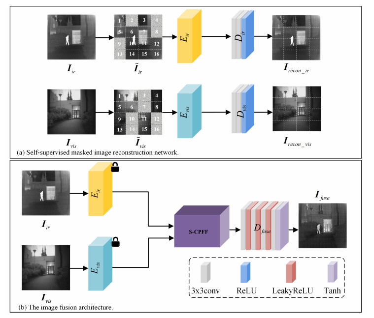
Infrared and visible image fusion (IVIF) is devoted to extracting and integrating useful complementary information from muti-modal source images. Current fusion methods usually require a large number of paired images to train the models in supervised or unsupervised way. In this paper, we propose CTFusion, a convolutional neural network (CNN)-Transformer-based IVIF framework that uses self-supervised learning. The whole framework is based on an encoder-decoder network, where encoders are endowed with strong local and global dependency modeling ability via the CNN-Transformer-based feature extraction (CTFE) module design. Thanks to the development of self-supervised learning, the model training does not require ground truth fusion images with simple pretext task. We designed a mask reconstruction task according to the characteristics of IVIF, through which the network can learn the characteristics of both infrared and visible images and extract more generalized features. We evaluated our method and compared it to five competitive traditional and deep learning-based methods on three IVIF benchmark datasets. Extensive experimental results demonstrate that our CTFusion can achieve the best performance compared to the state-of-the-art methods in both subjective and objective evaluations.
Citation: Keying Du, Liuyang Fang, Jie Chen, Dongdong Chen, Hua Lai. CTFusion: CNN-transformer-based self-supervised learning for infrared and visible image fusion[J]. Mathematical Biosciences and Engineering, 2024, 21(7): 6710-6730. doi: 10.3934/mbe.2024294
Infrared and visible image fusion (IVIF) is devoted to extracting and integrating useful complementary information from muti-modal source images. Current fusion methods usually require a large number of paired images to train the models in supervised or unsupervised way. In this paper, we propose CTFusion, a convolutional neural network (CNN)-Transformer-based IVIF framework that uses self-supervised learning. The whole framework is based on an encoder-decoder network, where encoders are endowed with strong local and global dependency modeling ability via the CNN-Transformer-based feature extraction (CTFE) module design. Thanks to the development of self-supervised learning, the model training does not require ground truth fusion images with simple pretext task. We designed a mask reconstruction task according to the characteristics of IVIF, through which the network can learn the characteristics of both infrared and visible images and extract more generalized features. We evaluated our method and compared it to five competitive traditional and deep learning-based methods on three IVIF benchmark datasets. Extensive experimental results demonstrate that our CTFusion can achieve the best performance compared to the state-of-the-art methods in both subjective and objective evaluations.

| [1] |
Y. Liu, X. Chen, Z. Wang, Z. Wang, R. K. Ward, X. Wang, Deep learning for pixel-level image fusion: Recent advances and future prospects, Inform. Fusion, 42 (2018), 158–173. https://doi.org/10.1016/j.inffus.2017.10.007 doi: 10.1016/j.inffus.2017.10.007

|
| [2] |
H. Zhang, H. Xu, X. Tian, J. Jiang, J. Ma, Image fusion meets deep learning: A survey and perspective, Inform. Fusion, 76 (2021), 323–336. https://doi.org/10.1016/j.inffus.2021.06.008 doi: 10.1016/j.inffus.2021.06.008
|
| [3] |
J. Ma, Y. Ma, C. Li, Infrared and visible image fusion methods and applications: A survey, Inform. Fusion, 45 (2019), 153–178. https://doi.org/10.1016/j.inffus.2018.02.004 doi: 10.1016/j.inffus.2018.02.004
|
| [4] |
C. Yang, J. Zhang, X. Wang, X. Liu, A novel similarity based quality metric for image fusion, Inform. Fusion, 9 (2008), 156–160. https://doi.org/10.1016/j.inffus.2006.09.001 doi: 10.1016/j.inffus.2006.09.001
|
| [5] | X. Zhang, P. Ye, G. Xiao, VIFB: a visible and infrared image fusion benchmark, in 2020 IEEE/CVF Conference on Computer Vision and Pattern Recognition Workshops (CVPRW), (2020), 468–478. https://doi.org/10.1109/CVPRW50498.2020.00060 |
| [6] | L. J. Chipman, T. M. Orr, L. N. Graham, Wavelets and image fusion, in International Conference on Image Processing, (1995), 248–251. https://doi.org/10.1109/ICIP.1995.537627 |
| [7] |
A. V. Vanmali, V. M. Gadre, Visible and NIR image fusion using weight-map-guided Laplacian-Gaussian pyramid for improving scene visibility, Sādhanā, 42 (2017), 1063–1082. https://doi.org/10.1007/s12046-017-0673-1 doi: 10.1007/s12046-017-0673-1
|
| [8] |
L. Sun, Y. Li, M. Zheng, Z. Zhong, Y. Zhang, MCnet: Multiscale visible image and infrared image fusion network, Signal Process., 208 (2023), 108996. https://doi.org/10.1016/j.sigpro.2023.108996 doi: 10.1016/j.sigpro.2023.108996
|
| [9] | K. He, X. Zhang, S. Ren, J. Sun, Deep residual learning for image recognition, in 2016 IEEE Conference on Computer Vision and Pattern Recognition (CVPR), (2016), 770–778. https://doi.org/10.1109/CVPR.2016.90 |
| [10] | J. Redmon, S. Divvala, R. Girshick, A. Farhadi, You only look once: Unified, real-time object detection, in 2016 IEEE Conference on Computer Vision and Pattern Recognition (CVPR), (2016), 779–788. https://doi.org/10.1109/CVPR.2016.91 |
| [11] | Y. Zhang, Y. Wang, H. Li, S. Li, Cross-compatible embedding and semantic consistent feature construction for sketch re-identification, in Proceedings of the 30th ACM International Conference on Multimedia, (2022), 3347–3355. https://doi.org/10.1145/3503161.3548224 |
| [12] |
H. Li, N. Dong, Z. Yu, D. Tao, G. Qi, Triple adversarial learning and multi-view imaginative reasoning for unsupervised domain adaptation person re-identification, IEEE Trans. Circuits Syst. Video Technol., 32 (2022), 2814–2830. https://doi.org/10.1109/TCSVT.2021.3099943 doi: 10.1109/TCSVT.2021.3099943
|
| [13] | O. Ronneberger, P. Fischer, T. Brox, U-Net: Convolutional networks for biomedical image segmentation, in Medical Image Computing and Computer-Assisted Intervention-MICCAI 2015, 9351 (2015), 234–241. https://doi.org/10.1007/978-3-319-24574-4_28 |
| [14] |
L. Tang, H. Huang, Y. Zhang, G. Qi, Z. Yu, Structure-embedded ghosting artifact suppression network for high dynamic range image reconstruction, Knowl.-Based Syst., 263 (2023), 110278. https://doi.org/10.1016/j.knosys.2023.110278 doi: 10.1016/j.knosys.2023.110278
|
| [15] |
H. Li, X. Wu, DenseFuse: A fusion approach to infrared and visible images, IEEE Trans. Image Process., 28 (2019), 2614–2623. https://doi.org/10.1109/TIP.2018.2887342 doi: 10.1109/TIP.2018.2887342
|
| [16] |
H. Li, J. Liu, Y. Zhang, Y. Liu, A deep learning framework for infrared and visible image fusion without strict registration, Int. J. Comput. Vision, (2024), 1625–1644. https://doi.org/10.1007/s11263-023-01948-x doi: 10.1007/s11263-023-01948-x
|
| [17] | L. Qu, S. Liu, M. Wang, Z. Song, Transmef: A transformer-based multi-exposure image fusion framework using self-supervised multi-task learning, preprint, arXiv: 2112.01030. |
| [18] | K. He, X. Chen, S. Xie, Y. Li, P. Dollár, R. Girshick, Masked autoencoders are scalable vision learners, in 2022 IEEE/CVF Conference on Computer Vision and Pattern Recognition (CVPR), (2022), 15979–15988. https://doi.org/10.1109/CVPR52688.2022.01553 |
| [19] |
S. Li, X. Kang, L. Fang, J. Hu, H. Yin, Pixel-level image fusion: A survey of the state of the art, Inform. Fusion, 33 (2017), 100–112. https://doi.org/10.1016/j.inffus.2016.05.004 doi: 10.1016/j.inffus.2016.05.004
|
| [20] |
H. Li, X. Qi, W. Xie, Fast infrared and visible image fusion with structural decomposition, Knowl.-Based Syst., 204 (2020), 106182. https://doi.org/10.1016/j.knosys.2020.106182 doi: 10.1016/j.knosys.2020.106182
|
| [21] |
Q. Zhang, Y. Liu, R. S. Blum, J. Han, D. Tao, Sparse representation based multi-sensor image fusion for multi-focus and multi-modality images: A review, Inform. Fusion, 40 (2018), 57–75. https://doi.org/10.1016/j.inffus.2017.05.006 doi: 10.1016/j.inffus.2017.05.006
|
| [22] |
M. Xie, J. Wang, Y. Zhang A unified framework for damaged image fusion and completion based on low-rank and sparse decomposition, Signal Process.: Image Commun., 98 (2021), 116400. https://doi.org/10.1016/j.image.2021.116400 doi: 10.1016/j.image.2021.116400
|
| [23] |
H. Li, Y. Wang, Z. Yang, R. Wang, X. Li, D. Tao, Discriminative dictionary learning-based multiple component decomposition for detail-preserving noisy image fusion, IEEE Trans. Instrum. Meas., 69 (2020), 1082–1102. https://doi.org/10.1109/TIM.2019.2912239 doi: 10.1109/TIM.2019.2912239
|
| [24] |
W. Xiao, Y. Zhang, H. Wang, F. Li, H. Jin, Heterogeneous knowledge distillation for simultaneous infrared-visible image fusion and super-resolution, IEEE Trans. Instrum. Meas., 71 (2022), 1–15. https://doi.org/10.1109/TIM.2022.3149101 doi: 10.1109/TIM.2022.3149101
|
| [25] |
Y. Zhang, M. Yang, N. Li, Z. Yu, Analysis-synthesis dictionary pair learning and patch saliency measure for image fusion, Signal Process., 167 (2020), 107327. https://doi.org/10.1016/j.sigpro.2019.107327 doi: 10.1016/j.sigpro.2019.107327
|
| [26] |
Y. Niu, S. Xu, L. Wu, W. Hu, Airborne infrared and visible image fusion for target perception based on target region segmentation and discrete wavelet transform, Math. Probl. Eng., 2012 (2012), 1–10. https://doi.org/10.1155/2012/275138 doi: 10.1155/2012/275138
|
| [27] |
D. M. Bulanon, T. F. Burks, V. Alchanatis, Image fusion of visible and thermal images for fruit detection, Biosyst. Eng., 103 (2009), 12–22. https://doi.org/10.1016/j.biosystemseng.2009.02.009 doi: 10.1016/j.biosystemseng.2009.02.009
|
| [28] |
M. Choi, R. Y. Kim, M. Nam, H. O. Kim, Fusion of multispectral and panchromatic satellite images using the curvelet transform, IEEE Geosci. Remote Sens. Lett., 2 (2005), 136–140. https://doi.org/10.1109/LGRS.2005.845313 doi: 10.1109/LGRS.2005.845313
|
| [29] |
Y. Liu, X. Chen, J. Cheng, H. Peng, Z. Wang, Infrared and visible image fusion with convolutional neural networks, Int. J. Wavelets, Multiresolution Inf. Process., 16 (2018), 1850018. https://doi.org/10.1142/S0219691318500182 doi: 10.1142/S0219691318500182
|
| [30] |
J. Ma, W. Yu, P. Liang, C. Li, J. Jiang, FusionGAN: A generative adversarial network for infrared and visible image fusion, Inform. Fusion, 48 (2019), 11–26. https://doi.org/10.1016/j.inffus.2018.09.004 doi: 10.1016/j.inffus.2018.09.004
|
| [31] |
H. Li, Y. Cen, Y. Liu, X. Chen, Z. Yu, Different input resolutions and arbitrary output resolution: A meta learning-based deep framework for infrared and visible image fusion, IEEE Trans. Image Process., 30 (2021), 4070–4083. https://doi.org/10.1109/TIP.2021.3069339 doi: 10.1109/TIP.2021.3069339
|
| [32] |
H. Zhang, J. Ma, SDNet: A versatile squeeze-and-decomposition network for real-time image fusion, Int. J. Comput. Vision, 129 (2021), 2761–2785. https://doi.org/10.1007/s11263-021-01501-8 doi: 10.1007/s11263-021-01501-8
|
| [33] |
H. Xu, J. Ma, J. Jiang, X. Guo, H. Ling, U2fusion: A unified unsupervised image fusion network, IEEE Trans. Pattern Anal. Mach. Intell., 44 (2020), 502–518. https://doi.org/10.1109/TPAMI.2020.3012548 doi: 10.1109/TPAMI.2020.3012548
|
| [34] |
L. Tang, J. Yuan, J. Ma, Image fusion in the loop of high-level vision tasks: A semantic-aware real-time infrared and visible image fusion network, Inform. Fusion, 82 (2022), 28–42. https://doi.org/10.1016/j.inffus.2021.12.004 doi: 10.1016/j.inffus.2021.12.004
|
| [35] | J. Liu, X. Fan, Z. Huang, G. Wu, R. Liu, W. Zhong, et al., Target-aware dual adversarial learning and a multi-scenario multi-modality benchmark to fuse infrared and visible for object detection, in 2022 IEEE/CVF Conference on Computer Vision and Pattern Recognition (CVPR), (2022), 5792–5801. https://doi.org/10.1109/CVPR52688.2022.00571 |
| [36] | A. Vaswani, N. Shazeer, N. Parmar, J. Uszkoreit, L. Jones, A. N. Gomez, et al., Attention is all you need, in Proceedings of the 31st International Conference on Neural Information Processing Systems, (2017), 6000–6010. |
| [37] | H. Chen, Y. Wang, T. Guo, C, Xu, Y. Deng, Z. Liu, et al., Pre-trained image processing transformer, in 2021 IEEE/CVF Conference on Computer Vision and Pattern Recognition (CVPR), (2021), 12294–12305. https://doi.org/10.1109/CVPR46437.2021.01212 |
| [38] | X. Zhu, W. Su, L. Lu, B. Li, X. Wang, J. Dai, Deformable DETR: Deformable transformers for end-to-end object detection, preprint, arXiv: 2010.04159. |
| [39] | S. Zheng, J. Lu, H. Zhao, X. Zhu, Z. Luo, Y. Wang, et al., Rethinking semantic segmentation from a sequence-to-sequence perspective with transformers, in 2021 IEEE/CVF Conference on Computer Vision and Pattern Recognition (CVPR), (2021), 6877–6886. https://doi.org/10.1109/CVPR46437.2021.00681 |
| [40] | A. Dosovitskiy, L. Beyer, A. Kolesnikov, D. Weissenborn, X. Zhai, T. Unterthiner, et al., An image is worth 16$\times$16 words: Transformers for image recognition at scale, in International Conference on Learning Representations ICLR 2021, (2021). |
| [41] | K. Han, A. Xiao, E. Wu, J. Guo, C. Xu, Y. Wang, Transformer in transformer, in 35th Conference on Neural Information Processing Systems (NeurIPS 2021), (2021), 1–12. |
| [42] | C. Chen, R. Panda, Q. Fan, RegionViT: Regional-to-local attention for vision transformers, preprint, arXiv: 2106.02689. |
| [43] | V. Vs, J. M. J. Valanarasu, P. Oza, V. M. Patel, Image fusion transformer, in 2022 IEEE International Conference on Image Processing (ICIP), (2022), 3566–3570. https://doi.org/10.1109/ICIP46576.2022.9897280 |
| [44] |
Y. Zhang, Y. Tian, Y. Kong, B. Zhong, Y. Fu, Residual dense network for image restoration, IEEE Trans. Pattern Anal. Mach. Intell., 43 (2021), 2480–2495. https://doi.org/10.1109/TPAMI.2020.2968521 doi: 10.1109/TPAMI.2020.2968521
|
| [45] |
R. Hou, D. Zhou, R. Nie, D. Liu, L. Xiong, Y. Guo, et al., VIF-Net: An unsupervised framework for infrared and visible image fusion, IEEE Trans. Comput. Imaging, 6 (2020), 640–651. https://doi.org/10.1109/TCI.2020.2965304 doi: 10.1109/TCI.2020.2965304
|
| [46] |
J. Liu, Y. Wu, Z. Huang, R. Liu, X. Fan, SMoA: Searching a modality-oriented architecture for infrared and visible image fusion, IEEE Signal Process. Lett., 28 (2021), 1818–1822. https://doi.org/10.1109/LSP.2021.3109818 doi: 10.1109/LSP.2021.3109818
|
| [47] |
Y. Zhang, Y. Liu, P. Sun, H. Yan, X. Zhao, L. Zhang, IFCNN: A general image fusion framework based on convolutional neural network, Inform. Fusion, 54 (2020), 99–118. https://doi.org/10.1016/j.inffus.2019.07.011 doi: 10.1016/j.inffus.2019.07.011
|
| [48] | H. Zhang, H. Xu, Y. Xiao, X. Guo, J. Ma, Rethinking the image fusion: A fast unified image fusion network based on proportional maintenance of gradient and intensity, in Proceedings of the AAAI Conference on Artificial Intelligence, 34 (2020), 12797–12804. https://doi.org/10.1609/aaai.v34i07.6975 |
| [49] |
H. Li, X. Wu, CrossFuse: A novel cross attention mechanism based infrared and visible image fusion approach, Inform. Fusion, 103 (2024), 102147. https://doi.org/10.1016/j.inffus.2023.102147 doi: 10.1016/j.inffus.2023.102147
|
| [50] |
H. Li, X. Wu, J. Kittler, RFN-Nest: An end-to-end residual fusion network for infrared and visible images, Inform. Fusion, 73 (2021), 72–86. https://doi.org/10.1016/j.inffus.2021.02.023 doi: 10.1016/j.inffus.2021.02.023
|
| [51] | M. Deshmukh, U. Bhosale, Image fusion and image quality assessment of fused images, Int. J. Image Process., 4 (2010), 484–508. |
| [52] |
H. Chen, P. K. Varshney, A human perception inspired quality metric for image fusion based on regional information, Inform. Fusion, 8 (2007), 193–207. https://doi.org/10.1016/j.inffus.2005.10.001 doi: 10.1016/j.inffus.2005.10.001
|
| [53] |
V. Aslantas, E. Bendes, A new image quality metric for image fusion: The sum of the correlations of differences, AEU-International J. Electron. Commun., 69 (2015), 1890–1896. https://doi.org/10.1016/j.aeue.2015.09.004 doi: 10.1016/j.aeue.2015.09.004
|
| [54] |
Z. Wang, A. C. Bovik, A universal image quality index, IEEE Signal Process. Lett., 9 (2002), 81–84. https://doi.org/10.1109/97.995823 doi: 10.1109/97.995823
|
| [55] | D. P. Kingma, J. Ba, Adam: A method for stochastic optimization, preprint, arXiv: 1412.6980. |
| [56] |
A. Toet, The TNO multiband image data collection, Data Brief, 15 (2017), 249–251. https://doi.org/10.6084/m9.figshare.1008029.v2 doi: 10.6084/m9.figshare.1008029.v2
|
| [57] | X. Jia, C. Zhu, M. Li, W. Tang, W. Zhou, LLVIP: A visible-infrared paired dataset for low-light vision, in 2021 IEEE/CVF International Conference on Computer Vision Workshops (ICCVW), (2021), 3489–3497. https://doi.org/10.1109/ICCVW54120.2021.00389 |
| [58] | K. A. Johnson, J. A. Becker, The Whole Brain, 2024. Available from: http://www.med.harvard.edu/AANLIB/home.html. |
| [59] |
H. Li, J. Zhao, J. Li, Z. Yu, G. Liu, Feature dynamic alignment and refinement for infrared–visible image fusion: Translation robust fusion, Inform. Fusion, 95 (2023), 26–41. https://doi.org/10.1016/j.inffus.2023.02.011 doi: 10.1016/j.inffus.2023.02.011
|


Figures(9) / Tables(5)

Keying Du, Liuyang Fang, Jie Chen, Dongdong Chen, Hua Lai. CTFusion: CNN-transformer-based self-supervised learning for infrared and visible image fusion[J]. Mathematical Biosciences and Engineering, 2024, 21(7): 6710-6730. doi: 10.3934/mbe.2024294


 DownLoad: