Adaptive dynamic self-learning grey wolf optimization algorithm for solving global optimization problems and engineering problems

Yijie Zhang; Yuhang Cai; Yijie Zhang; Yuhang Cai

doi:10.3934/mbe.2024174

Mathematical Biosciences and Engineering

2024, Volume 21, Issue 3: 3910-3943. doi: 10.3934/mbe.2024174

Previous Article Next Article

Research article

Adaptive dynamic self-learning grey wolf optimization algorithm for solving global optimization problems and engineering problems

Yijie Zhang ,
Yuhang Cai ^,

School of Artificial Intelligence and Computer Science, Jiangnan University, WuXi 214122, China

Received: 30 January 2024 Revised: 14 February 2024 Accepted: 18 February 2024 Published: 21 February 2024

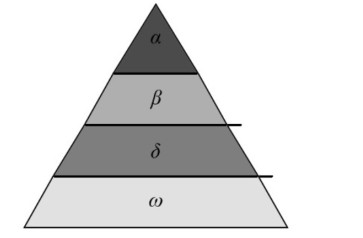
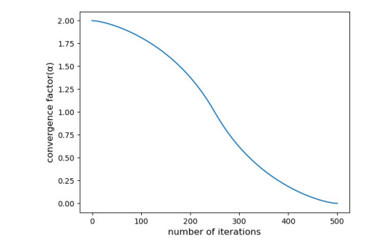
The grey wolf optimization algorithm (GWO) is a new metaheuristic algorithm. The GWO has the advantages of simple structure, few parameters to adjust, and high efficiency, and has been applied in various optimization problems. However, the orginal GWO search process is guided entirely by the best three wolves, resulting in low population diversity, susceptibility to local optima, slow convergence rate, and imbalance in development and exploration. In order to address these shortcomings, this paper proposes an adaptive dynamic self-learning grey wolf optimization algorithm (ASGWO). First, the convergence factor was segmented and nonlinearized to balance the global search and local search of the algorithm and improve the convergence rate. Second, the wolves in the original GWO approach the leader in a straight line, which is too simple and ignores a lot of information on the path. Therefore, a dynamic logarithmic spiral that nonlinearly decreases with the number of iterations was introduced to expand the search range of the algorithm in the early stage and enhance local development in the later stage. Then, the fixed step size in the original GWO can lead to algorithm oscillations and an inability to escape local optima. A dynamic self-learning step size was designed to help the algorithm escape from local optima and prevent oscillations by reasonably learning the current evolution success rate and iteration count. Finally, the original GWO has low population diversity, which makes the algorithm highly susceptible to becoming trapped in local optima. A novel position update strategy was proposed, using the global optimum and randomly generated positions as learning samples, and dynamically controlling the influence of learning samples to increase population diversity and avoid premature convergence of the algorithm. Through comparison with traditional algorithms, such as GWO, PSO, WOA, and the new variant algorithms EOGWO and SOGWO on 23 classical test functions, ASGWO can effectively improve the convergence accuracy and convergence speed, and has a strong ability to escape from local optima. In addition, ASGWO also has good performance in engineering problems (gear train problem, ressure vessel problem, car crashworthiness problem) and feature selection.

Keywords:

Citation: Yijie Zhang, Yuhang Cai. Adaptive dynamic self-learning grey wolf optimization algorithm for solving global optimization problems and engineering problems[J]. Mathematical Biosciences and Engineering, 2024, 21(3): 3910-3943. doi: 10.3934/mbe.2024174

Related Papers:

[1]	Wenqiang Zhang, Chen Li, Mitsuo Gen, Weidong Yang, Zhongwei Zhang, Guohui Zhang . Multiobjective particle swarm optimization with direction search and differential evolution for distributed flow-shop scheduling problem. Mathematical Biosciences and Engineering, 2022, 19(9): 8833-8865. doi: 10.3934/mbe.2022410
[2]	Shiqi Zou, Xiaoping Shi, Shenmin Song . A multi-objective optimization framework with rule-based initialization for multi-stage missile target allocation. Mathematical Biosciences and Engineering, 2023, 20(4): 7088-7112. doi: 10.3934/mbe.2023306
[3]	Ruiping Yuan, Jiangtao Dou, Juntao Li, Wei Wang, Yingfan Jiang . Multi-robot task allocation in e-commerce RMFS based on deep reinforcement learning. Mathematical Biosciences and Engineering, 2023, 20(2): 1903-1918. doi: 10.3934/mbe.2023087
[4]	Rongmei Geng, Renxin Ji, Shuanjin Zi . Research on task allocation of UAV cluster based on particle swarm quantization algorithm. Mathematical Biosciences and Engineering, 2023, 20(1): 18-33. doi: 10.3934/mbe.2023002
[5]	Yanpei Liu, Yunjing Zhu, Yanru Bin, Ningning Chen . Resources allocation optimization algorithm based on the comprehensive utility in edge computing applications. Mathematical Biosciences and Engineering, 2022, 19(9): 9147-9167. doi: 10.3934/mbe.2022425
[6]	Haolan Zhou, Gang Chen, Yujun Lu, Xiaoya Cheng, Hao Xin . A permutation-combination heuristics for crane-based automated storage and retrieval systems considering order fulfillment time and energy consumption. Mathematical Biosciences and Engineering, 2024, 21(1): 116-143. doi: 10.3934/mbe.2024006
[7]	Rui Zhu, Yuhang Chen, Qianqian Yu, Siqing Liu, Jianjie Wang, Zhili Zeng, Liming Cheng . Effects of contusion load on cervical spinal cord: A finite element study. Mathematical Biosciences and Engineering, 2020, 17(3): 2272-2283. doi: 10.3934/mbe.2020120
[8]	Begoña González, Daniel A. Rossit, Máximo Méndez, Mariano Frutos . Objective space division-based hybrid evolutionary algorithm for handing overlapping solutions in combinatorial problems. Mathematical Biosciences and Engineering, 2022, 19(4): 3369-3401. doi: 10.3934/mbe.2022156
[9]	Smita Shandilya, Ivan Izonin, Shishir Kumar Shandilya, Krishna Kant Singh . Mathematical modelling of bio-inspired frog leap optimization algorithm for transmission expansion planning. Mathematical Biosciences and Engineering, 2022, 19(7): 7232-7247. doi: 10.3934/mbe.2022341
[10]	Bin Deng, Ran Ding, Jingfeng Li, Junfeng Huang, Kaiyi Tang, Weidong Li . Hybrid multi-objective metaheuristic algorithms for solving airline crew rostering problem with qualification and language. Mathematical Biosciences and Engineering, 2023, 20(1): 1460-1487. doi: 10.3934/mbe.2023066

Abstract

1. Introduction

Online sourcing of fresh food for daily needs has grown in popularity as a way to avoid human contact in public places and reduce the risk of infection during epidemics. Farmers' markets have moved to e-commerce platforms, and fresh food retail e-commerce has emerged as a popular new retail type ^[1]. The impact of the epidemic will continue to accelerate the development of fresh food e-commerce in the future, with the fresh food e-commerce industry expected to exceed a trillion yuan in 2023, with a high growth trend ^[2]. There are three major forms of logistics network and operational models in the retail form of fresh food e-commerce: (1) Front warehouse mode. Fresh e-commerce platforms set up multiple small warehouses (front warehouses) near communities where consumers are concentrated, and couriers provide customers with instant delivery service from these front warehouses ^[3]. (2) Warehouse and store integration mode. The store serves as a small fresh food supermarket and fulfills online orders. Consumers can purchase from the store or place orders online, with express delivery ^[4]. (3) Community group buying mode. Fresh e-commerce initiates group purchases, summarizes orders and distributes products to customers in the community through group buying leaders, while the fresh platform is responsible for the procurement, transportation and after-sales service of fresh food ^[5].

Front warehouse mode can solve the last mile problem and ensure freshness and timely delivery ^[6], and it is distinguished from the other two e-commerce modes by its small scale, proximity to the consumer, high layout density and efficient distribution ^[7]. However, compared to the other two operating modes, front warehouse mode increases the length of the supply chain and incurs higher fulfillment costs (including warehouse rent, inventory costs and order delivery costs), which have become one of the main bottlenecks restricting the development of fresh e-commerce corporations operating in front warehouse mode ^[8]. Consequently, research on the location optimization of fresh food e-commerce front warehouses is of great application value. This paper presents a case study of an e-commerce company locating new locations for front warehouses using a location optimization model with the goal of minimizing total distribution system cost. The location and allocation decision of front warehouses can be described as follows: In the given set of alternative front warehouse and customer locations, select a certain number to open according to the distribution of customer locations and the quantity of demand, and allocate the customer orders to the open front warehouses nearby, to ensure optimal cost of the distribution network.

The remainder of the paper is structured as follows. Section 2 is a review of the literature. Section 3 discusses the problem description, assumptions and mathematical model. Section 4 presents the solution approach, Section 5 gives a real case study, and Section 6 concludes the paper with limitations and recommendations for future research.

2. Literature review

2.1. Research on sustainable closed loop supply chain network and location problem

The concepts of sustainable development and circular economy have received extensive attention. Scholars delve into sustainable closed-loop supply chain networks, and have adopted sustainability factors, such as carbon emission, energy consumption and environmental pollution, into their research to respond to real challenges ^[9]. Goodarzian et al. investigated a citrus fruit supply chain network in Iran to minimize the total cost and CO₂ emission simultaneously ^[10]. Momenitabar et al. designed a sustainable bioethanol supply chain network to cope with the demand increase of bioethanol ^[11]. Fresh food requires low-temperature preservation during transportation, which greatly meets the quality requirements of consumers but also creates huge energy consumption and carbon emissions ^[12]. Therefore, research on the sustainability of cold chain transportation is particularly important. Govindan et al. ^[13] and Wang et al. ^[14] both studied the cold chain location and routing problem (VRP) from the perspective of low carbon and environmental protection to minimize the impact of carbon emissions on the environment. Wang et al. constructed a bi-objective model to realize carbon emission reduction in fresh agricultural cold chain logistics ^[15]. Liu designed a dynamic model to reflect the carbon emission cost affected by time-varying vehicle speed ^[16].

Specifically, scholars have basically matured their research methods on the e-commerce warehouse location problem, mainly based on quantitative analysis, which quantifies costs, service level, demand, time window and other elements to formulate a location model, with designs of specific algorithms to solve it. For example, Nuno et al. presented a solution for selecting a location for the installation of an e-commerce warehouse with the goals of lowering logistics costs and ensuring service improvements, and the problem was solved using multiple criteria decision-making ^[17]. Wang used the effective covering model to conduct an empirical analysis on the location selection problem of marine product e-commerce distribution centers, taking into account factors such as the surrounding environment, public facilities and population ^[18]. Ahmadi et al. established a mixed integer programming location model with the goal of maximizing the total profit of serving customers, considering the price elasticity of demand ^[19]. Macedo et al. proposed a heuristic algorithm based on skewed universal variable neighborhood search to solve the VRP for perishable goods with time constraints ^[20].

2.2. Research on algorithms of location model

Both precise and heuristic algorithms can solve location problems. The former is suitable for situations where the problem size is not large and can obtain the optimal solution. When the scale of the problem is large, heuristic algorithms can efficiently obtain the Pareto optimization. The location problem is a classic NP-hard problem, and the Pareto optimal solution of an instance can be obtained using heuristic algorithms ^[21]. Torabi et al. proposed a new fuzzy-stochastic hybrid programming model based on two-stage scenarios and designed an effective multi-step solution to solve practical problems ^[22]. Erdin and Akbas took the location of storage facilities as a multi-criteria problem, and applied multi-criteria decision-making and TOPSIS (technique for order preference by similarity to an ideal solution) method to plan the location of storage facilities ^[23]. Silva et al. used three linear relaxation heuristic algorithms and genetic algorithm combined with variable neighborhood hybrid algorithm to solve the problem. The research showed that the performance of the hybrid algorithm was better than the linear relaxation heuristic algorithm ^[24]. Considering random demand, Silva et al. designed location models for internal distribution and outsourcing operation strategies of e-commerce enterprises, and carried out accurate solutions and heuristic solutions for the models, respectively ^[25].

2.3. Research gaps

Most of the literature only considers the process from front warehouses to customers, neglecting the process from urban distribution center to front warehouses. The improvement of distribution efficiency of a logistics system involves every circulation of the supply chain. This paper takes the front warehouse location problem as a three-tier two-stage logistics network. Although there is extensive research on fresh food e-commerce, the research in specific fields is limited, especially the quantitative research on front warehouse location. The main difference is that the front warehouse of fresh food e-commerce studied in this paper is the end node in the logistics process, providing last-mile service, with a small service scope and scattered service objects. Therefore, it is necessary to finely depict practical problems and systematically consider factors such as cost and environment.

2.4. Contribution

This work presents two major contributions. First, a model of front warehouse location with the objective of total minimum cost is established, and the model and case study make a detailed description of the location of the front warehouse and comprehensive consideration of the location cost. Second, the improved immune algorithm is applied to solve the model, and the comparison with GA proves the validity of the proposed algorithm. Also, a real case study shows that the proposed algorithm is better in performance than the traditional genetic algorithm, and the real case study gives a reference for optimizing the layout of a front warehouse for fresh food e-commerce enterprises. In a word, the research of this study is of practical and academical significance.

3. Front warehouse location allocation model

3.1. Problem description

Figure 1 depicts the operating mode of a fresh produce e-commerce business with forward warehouses, which includes a point of origin, regional warehouses, front warehouses and customer points. Regional warehouses are large warehouses that are set up for each province or city, with good cold chain storage and processing facilities, and they are typically located far from urban centers. Front warehouses are typically located within the city or in densely populated areas of the city, making it easier to deliver fresh goods to customers in a shorter period of time. First, the e-commerce company buys fresh produce directly from the source and transports it to a regional warehouse where it is processed and packaged. The fresh goods are then transported to front warehouses, where they are temporarily stored to fulfill customer orders. When a customer order is received, the front warehouse with available stock will fulfill the order quickly. To meet the needs of consumers, two specific issues should be addressed. To begin with, in order to make profit, the goal is to reduce total delivery cost. Furthermore, all demand points should be covered. This model divides logistics distribution into two phases: First, products are supplied from urban distribution centers to front warehouses, and then, products are delivered from front warehouses to consumers.

Figure 1. Fresh food e-commerce network with front warehouses.

DownLoad: Full-Size Img PowerPoint

3.2. Problem hypothesis

Before developing a model, the following assumptions are made in order to solve the problems listed above:

(1) Only choose the front warehouse from the list of alternative addresses.

(2) Distribution vehicles have the same model and limited capacity.

(3) The operating costs of front warehouses and vehicles are not taken into account.

(4) Customer service time, and loading and unloading time are not taken into account.

(5) Only one supply point can serve a front warehouse, and two or more front warehouses cannot serve a demand point at the same time.

(6) Maintain a constant temperature throughout the delivery process.

(7) Vehicles travel at a fixed value.

3.3. Parameter description

The following are the definitions of the model's parameters.

$I\left\{i|i = \mathrm{1, 2}, \cdots, I\right\}$ : set of candidate front warehouses;

$J\left\{j|j = \mathrm{1, 2}, \cdots, \mathrm{J}\right\}$ : set of demand points;

$L\left\{l|l = \mathrm{1, 2}, \cdots, L\right\}$ : set of vehicles;

$K\left\{k|k = \mathrm{1, 2}, \cdots, K\right\}$ : set of supply vendors;

${C}_{i}$ : fixed costs for establishing a front warehouse in area i;

$C$ : total cost for establishing a front warehouse;

$V$ : capacity of vehicle;

${T}_{o}$ : outdoor ambient temperature;

${T}_{r}$ : refrigeration temperature;

$\lambda$ : energy consumption factor;

${\alpha }_{1}$ : unit transportation cost from supplier to front warehouse;

${\alpha }_{2}$ : unit transportation cost from front warehouse to demand point;

${d}_{ki}$ : distance from supply vendor $k$ to front warehouse $i$ ;

${d}_{ij}$ : distance from front warehouse $i$ to demand point $j$ ;

${q}_{k}$ : supply quantity of vendor k;

${q}_{ki}$ : cargo volume from supply vendor $k$ to front warehouse $i$ ;

${q}_{ij}$ : demand from front warehouse $i$ to demand point $j$ ;

${P}_{j}$ : demand of point $j$ ;

$s$ : speed of vehicle;

${t}_{ki}$ : time of vehicle traveling from supply vendor $k$ to front warehouse $i$ ;

${t}_{ij}$ : time of vehicle traveling from front warehouse $i$ to demand point $j$ ;

${X}_{i}:{X}_{i} =$ 1 means $i\left(i\in I\right)$ is selected as front warehouse: for others, ${X}_{i} =$ 0;

${x}_{kil}:{x}_{kil} =$ 1 means vehicle $l$ transporting from supply vendor $k$ to front warehouse $i$ ;

for others, ${x}_{ijl} =$ 0;

${x}_{ijl}:{x}_{ijl} =$ 1 means vehicle $l$ transporting from front warehouse $i$ to demand point $j$ ;

for others, ${x}_{ijl} =$ 0;

${y}_{ij}:{y}_{ij} =$ 1 means demand point $j$ is served by front warehouse $i$ ;

for others, ${y}_{ij} =$ 0.

3.4. Model formulation

The front warehouse location allocation problem (FWLAP) model for fresh food logistics constructed in this paper takes the minimum total cost as the objective function. First, the components of the objective function are analyzed, and then the specific composition of the FWLAP model is determined.

3.4.1. Analysis of objective function

(1) Infrastructure and operating costs of fresh logistics distribution system

The infrastructure cost of the fresh food logistics distribution system mainly includes the purchase cost of land, the construction cost of the front warehouse distribution center, the salary and management expenses of workers employed by the distribution center and the expenses incurred by water and electricity consumption. The facility cost is

${C}_{1} = \sum _{i = 1}^{I}{X}_{i}{C}_{i}$

(1)

(2) Fresh logistics distribution and transportation cost

The transportation cost of fresh food logistics and distribution includes the transportation cost from the supply point to the distribution point and cost from the distribution point to the demand point. The total transportation and distribution cost of the two stages is

${C}_{2} = \sum _{i = 1}^{I}\sum _{k = 1}^{K}{d}_{ki}{q}_{ki}{{x}_{kil}\alpha }_{1}+\sum _{i = 1}^{I}\sum _{j = 1}^{J}{d}_{ij}{q}_{ij}{{x}_{ijl}\alpha }_{2}$

(2)

(3) Energy consumption cost

It is well known that vehicles loaded with fresh products need to keep the fresh products in a low-temperature environment during the distribution process. Compared to ordinary vehicles, fresh vehicles consume much more energy. The low-temperature environment of fresh vehicles requires fuel and power consumption to maintain, and the temperature of fresh vehicles is determined by the product type. The fuel and power consumption of different types of products are also different. If the outdoor ambient temperature is below zero, there is no need to refrigerate fresh foods such as vegetables and fruits, and the energy consumption cost will be very low.

${C}_{3} = \lambda \left(\sum _{i = 1}^{I}\sum _{k = 1}^{K}{d}_{ki}{q}_{ki}{x}_{kil}+\sum _{i = 1}^{I}\sum _{j = 1}^{J}{d}_{ij}{q}_{ij}{x}_{ijl}\right)$

(3)

where $\lambda = \left\{\begin{array}{c}0, {T}_{o}\le {T}_{r}\\ constants, {T}_{o} < {T}_{r}\end{array}\right.$ , ${T}_{o}$ is outdoor ambient temperature, and ${T}_{r}$ is reefertemperature required.

3.4.2. FWLAP model formulation

Through detailed analysis of the targets, the FWLAP model is formulated as follows:

${min\ C = }{C}_{1}+{C}_{2}+{C}_{3}$

(4)

s.t.

$\sum _{i\in I}{X}_{i}{C}_{i}\le C$

(5)

$\sum _{i\in I}{q}_{ki}\le {q}_{k}$

(6)

$\sum _{k\in K}{q}_{ki} = \sum _{j\in J}{q}_{ij}\ \ i\in I$

(7)

$\sum _{i\in I}{q}_{ij}\ge \sum _{i\in I}{r}_{j}\ \ i\in I$

(8)

$\sum _{i\in I}{X}_{i}\ge 1$

(9)

${q}_{ki} = \sum _{{i}^{'}\in \left\{i\right\}\cup J}\sum _{j\in J}\sum _{k\in K}{P}_{j}{x}_{{i}^{'}jk}\ \ \ \ i\in I$

(10)

${x}_{ijl} = 0\ \ \ \ i\in I, j\in J, l\in L$

(11)

${\sum }_{i\in I}{x}_{ijl}\le 1\ \ \ \ j\in J, l\in L$

(12)

${\sum }_{j\in I\cup J}{x}_{ijl}-{\sum }_{j\in I\cup J}{x}_{jil} = 0\ \ \ \ i\in I\cup J, l\in L$

(13)

${\sum }_{j\in J, i\in I\cup J}{x}_{ijl}\cdot {P}_{j}\le {V}_{l}\ \ \ \ l\in L$

(14)

${\sum }_{i, j\in I\cup J}{\sum }_{l\in L}{x}_{ijl}\ge 1$

(15)

${\sum }_{j\in J}{\sum }_{l\in L}{x}_{ijl}\ge {X}_{i}\ \ \ \ i\in I$

(16)

${\sum }_{j\in J}{x}_{ijl}\le {X}_{i}\ \ \ \ i\in I, l\in L$

(17)

${\sum }_{i\in I}{y}_{ij} = 1\ \ \ \ j\in J$

(18)

$\begin{array}{c} {X}_{i} = \mathrm{0, 1}\ \ \ \ i\in I \\ {x}_{kil} = \mathrm{0, 1}, {x}_{ijl} = \mathrm{0, 1}\ \ \ \ i, j\in I\cup J, l\in L, k\in K{y}_{ij} = \mathrm{0, 1}\ \ \ \ i\in I, j\in J \end{array}$

(19)

The goal of Eq (4) is to minimize total cost. Formula (5) indicates that the cost of the selected front warehouse cannot exceed the total cost of the front warehouse. Formula (6) means that the quantity of goods provided by a supplier to a front warehouse cannot exceed its supply capacity. Formula (7) displays that the goods in the front warehouse cannot be retained and are all used for distribution. Formula (8) indicates that the requirements of the demand point must be satisfied. Formula (9) indicates that there is at least one front warehouse. Equation (10) requires that the total front warehouse supply is equal to the total demand of the customer points. According to Eq (11), there is no lateral transportation of goods between front warehouses. Equation (12) represents that a vehicle is assigned to one of the front warehouses. Equation (13) ensures that the vehicle transportation path remains continuous. The capacity limit of vehicles is represented by Eq (14). Equation (15) indicates that a demand point can be served by multiple delivery vehicles. Equations (16) and (17) show that vehicles are only assigned to open front warehouses. Equation (18) represents that only one front warehouse serves a demand point. The constraints of decision variables are represented by Eq (19).

4. Immune optimization algorithm

4.1. Algorithm overview

There are numerous methods for resolving location issues, including analytical methods, optimal planning methods, comprehensive factor evaluation methods and so on. These methods, however, have limitations. The analytical method is limited to one distribution center location model. Although there is no limit on the number of distribution centers, the optimal planning method is not appropriate for complex models. The result of the comprehensive factor evaluation method is subjective. As a result, the proposed model is solved using a heuristic algorithm in this study. The genetic algorithm, immune algorithm and neural network are examples of intelligent optimization algorithms that are refined through repeated experimental simulations under various conditions or variants. Among them, immune algorithm research began in the 1980s, and research results show that it outperforms the classical genetic algorithm in solving location problems ^[26]. In this study, the immune algorithm is used to solve the proposed model.

The immune algorithm is an intelligent optimization algorithm that is generated by simulating the body's powerful immune system ^[27]. The biological immune system has powerful learning ability, recognition and memory ability to identify harmful information from the outside world, analyze the information and activate defense mechanisms to minimize system damage and ensure robustness and safety. The immune optimization algorithm uses the immune system's diversity generation and retention mechanism to maintain population diversity, overcoming the problem of "premature maturity" that is difficult to solve in the process of finding the optimal solution and successfully obtaining the global optimal solution.

4.2. Algorithm implementation steps

The flow chart of the immune algorithm is shown in Figure 2.

Figure 2. Flow chart of immune algorithm.

DownLoad: Full-Size Img PowerPoint

Step 1: Problem analysis. The goal of the research is to select several suitable locations from multiple alternatives in order to establish front warehouses with the shortest total distribution time.

Step 2: Antigen identification. The magnitude of the affinity between the antibody and the antigen is used to identify it.

Step 3: Generation of initial antibody population.

Step 4: Determine the expected probability of reproduction for each individual and evaluate each one in the population.

Step 5: Rank all individuals based on their expected reproduction probability, then choose the top N to form the parent population, and select the top m to store in the memory.

Step 6: Check to see if the loop termination condition is met. To complete the iterative loop, the maximum number of iterations is used as the termination condition.

Step 7: Generation of new population. Generation is made up of two parts, one obtained through antibody selection, crossover and mutation operations, and the other is obtained from the memory bank. After the new generation is generated, the cyclic operation continues.

The specific calculations used in the implementation of the immunization algorithm are as follows.

(1) Generation of the initial antibody population

If the memory bank is empty, the first antibody population is chosen at random from the feasible solution space. If the memory bank is not empty, then the initial antibody population is chosen from it. The initial antibody population in this paper is generated at random using simple coding, and different antibodies indicate different location schemes. The number of front warehouses determines the antibody length in this study, and the antibodies represent the set of selected front warehouses. For example, if there are 5 alternatives, 2 of them should be chosen to establish front warehouses, and antibodies ^[2,3] indicate that locations 2 and 3 are to open as front warehouses.

(2) Affinity calculation

The degree of recognition of an antigen by an antibody is expressed by the affinity between the antibody and the antigen. The expression of affinity function is as follows.

${A}_{v} = \frac{1}{{F}_{v}}$

(20)

where ${F}_{v}$ is the objective function of front warehouse location.

The affinity between antibodies and antibodies is used to measure their similarity, and the algorithm employs Forrest's R-site contiguity method. The principle of the R-site contiguity method is based on the partial matching rule, and the key is determining the R-value. If two individuals are coded with consecutive R-positions or more than R-positions, the antibodies are similar, and vice versa. In this paper, the following formula is used to calculate the antibody affinity.

${S}_{v, s} = \frac{{k}_{v, s}}{L}$

(21)

${k}_{v, s}$ denotes the same number of digits between antibodies v and s. L means the length of the antibody, and the value of L is determined by the number of the front warehouse selected. For example, two antibodies are [237854] and [438961], and the comparison shows that three same values exist for the two antibodies. Then the affinity is 0.5.

(3) Calculation of antibody concentration

Antibody concentration denotes the proportion of similar antibodies to the total number of antibodies in the population and characterizes antibody strength. When an external antigen or a new antibody attacks the immune system, the body's immune response becomes intense, and the number of antibodies changes. Most antibodies' affinity will increase as more antibodies are produced. When it exceeds a certain threshold, their concentration suffers. The formula for calculating antibody concentration is as follows.

${C}_{v} = \frac{1}{N}\sum _{j\in N}{S}_{v, s}$

(22)

where N denotes the total number of antibodies, and ${S}_{v, s}$ is a binary variable. ${S}_{v, s}$ = 1 when ${S}_{v, s}$ > T, and otherwise, ${S}_{v, s}$ = 0. T is a predetermined threshold value.

(4) Expected probability of reproduction

The expected reproduction probability P for each individual is determined by the antibody concentration and the affinity between the antibody and the antigen. The expression for calculating the expected reproduction probability is as follows.

$P = \alpha \frac{{A}_{v}}{\sum {A}_{v}}+(1-\alpha )\frac{{C}_{v}}{\sum {C}_{v}}$

(23)

The above equation shows that an individual's fitness is proportional to the expected reproductive probability, whereas individual concentration is inversely proportional to the desired reproduction probability. This suppresses the production of individuals with high concentration while promoting the production of individuals with high fitness, ensuring the population's diversity. $\alpha$ is a constant value.

(5) Immunization operation

Selection operation. The selection operation is carried out using a roulette selection mechanism. The probability of an individual being selected is determined by the ratio of an individual's expected reproductive probability to the overall.

Crossover operation. A crossover operation is one in which genes or gene segments from two chromosomes are exchanged in a specific manner to create a new individual. This paper chooses the crossover operation by multi-point crossover to make the good genes of the parents be inherited in order to produce new good individuals.

Mutation operation. The antibodies are drawn at random from the antibody population generated by the crossover operation, and one of the antibodies is mutated to create a new individual. The most commonly used mutation operations in practice are basic position mutation, flip mutation, adaptive crossover mutation, and so on. In this paper, the flip mutation operation is used to ensure population diversity. The new antibody population produced by the mutation operation is combined with the previously memorized one from memory.

4.3. Implementation of improved immunization algorithm

Because the traditional immune optimization algorithm conservatively retains the excellent individuals within the memory bank, the population quality improves as the number of iterations increases, but it is unable to retain more excellent individuals, resulting in a slower convergence rate, which affects computational accuracy. This paper proposes an improved immune algorithm to retain dynamically excellent individuals by establishing the dynamic retention mechanism. The number of excellent individual m in the memory bank is set to change dynamically, and the number of excellent individuals is preserved to increase as the population's overall quality improves. The m population quality function is presented as

$m = \frac{(\sum _{i = 1}^{p}{d}_{i}-p)}{p\times q}\times k$

(24)

where p is the number of demand points, q is the number of distribution centers, k is the size of the memory bank, and ${d}_{i}$ is the descending position of the distance between nodes in the set of distances between demand points and temporary distribution stations.

Traditional immunization relies on a certain probability to retain the best individual, which increases the number of iterations and computational effort while also affecting computational accuracy. As a result, the population in this paper is chosen using the Metropolis criterion. The i-th individual in a population is compared to the (i+1)-th, and the rule of accepting the (i+1)-th individual is chosen as in Eq (18); otherwise, the i-th individual is accepted.

$\left\{\begin{array}{c}{g}_{i+1}\left(x\right)\le {g}_{i}\left(x\right)\\ R\le exp\left(\frac{-{g}_{i+1}\left(x\right)-{g}_{i+1}\left(x\right)}{W}\right)\end{array}\right.$

(25)

where $g\left(x\right)$ denotes the fitness value, w is the temperature constant and R represents a random number uniformly distributed on [0, 1].

5. Case study

5.1. Basic data

5.1.1. Data of alternative front warehouses and urban distribution center

Alternative front warehouses make use of open areas near residential areas, such as city squares, stadiums, and open spaces. There are 15 open areas in Handan with available floor space of about 2000 m² that were chosen through field research and big data from e-map. Table 1 shows the data for each candidate front warehouse, including capacity, coordinates and available area. The amount of fresh produce that could be accommodated in the alternative temporary front warehouses was calculated assuming that the height of the temporary front warehouses ranged from 4 to 6 meters, and the storage capacity was 1000 kg per 7 cubic meters. The distribution mode is multi-vehicle distribution, in which vehicles begin at the distribution point proceed directly to the demand point, and return to the distribution point once the task is completed.

Table 1. Data of candidate front warehouses.

No.	Capacity/kg	Coordinates	Available area/m²	Infrastructure and operating costs
1	2714285	114.509175, 36.662958	6800	95520
2	5089285	114.500767, 36.654475	10,180	185,450
3	4571428	114.528543, 36.644384	8305	109,520
4	4007142	114.568266, 36.661235	8000	98,560
5	1600000	114.520637, 36.631519	2800	52,860
6	1714285	114.550461, 36.63023	2400	49,250
7	2857142	114.528071, 36.616084	4200	68,590
8	5714285	114.495117, 36.60505	8200	108,690
9	7000000	114.48475, 36.58346	9800	178,520
10	8571428	114.513137, 36.576953	12,000	205,130
11	8214285	114.47194, 36.655803	8200	90,250
12	3428571	114.475102, 36.634031	4800	75,520
13	1714285	114.45936, 36.619397	2400	60,250
14	3000000	114.451845, 36.615599	6300	85,020
15	6571428	114.438034, 36.572769	11,500	199,650

| Show Table

DownLoad: CSV

Location of the urban distribution center is set on the west side of the city with a capacity of 40,000 tons, which is currently the largest integrated cold storage in Handan city. Its geographical coordinates are (114.455441, 36.636189).

The layout of alternative front warehouses that meet the floor area of above 2000 m² is shown in Figure 3.

Figure 3. Layout of alternative front warehouses.

DownLoad: Full-Size Img PowerPoint

5.1.2. Data of demand points

The main urban area of the city Handan is subdivided into 86 demand points based on its geographical characteristics and population distribution, and the population number of each demand point is obtained from city statistics. Assuming a daily demand for fresh food of 2 kg per person, the daily demand is then calculated using the population number, and the specific data are shown in Table 2.

Table 2. Data of demand points.

No.	Coordinate of demand point	Qty of demand/kg	No.	Coordinate of demand point	Qty of demand/kg
1	114.548251, 36.646802	28,534	44	114.532801, 36.596083	21,816
2	114.534741, 36.651898	8076	45	114.52048, 36.597068	37,516
3	114.526908, 36.65572	9422	46	114.510451, 36.600835	13,986
4	114.517996, 36.656762	10,436	47	114.502761, 36.601994	29,848
5	114.508223, 36.656936	12,010	48	114.494569, 36.602863	30,114
6	114.495718, 36.658036	16,078	49	114.487526, 36.603558	28,366
7	114.495647, 36.647902	32,584	50	114.486448, 36.596663	24,314
8	114.509013, 36.643095	33,982	51	114.494137, 36.596489	14,476
9	114.52662, 36.645644	14,694	52	114.502689, 36.595561	20,388
10	114.493634, 36.63962	32,598	53	114.510019, 36.594808	15,890
11	114.524752, 36.636029	28,848	54	114.516703, 36.58484	20,212
12	114.536537, 36.635045	18,492	55	114.509085, 36.587216	30,808
13	114.548251, 36.634813	15,112	56	114.501539, 36.587796	38,202
14	114.563918, 36.625661	1108	57	114.488029, 36.591737	24,830
15	114.550407, 36.625545	28,416	58	114.503049, 36.578464	34,030
16	114.53431, 36.626704	42,264	59	114.492988, 36.583912	27,780
17	114.522596, 36.627804	27,464	60	114.482927, 36.587042	36,682
18	114.513182, 36.628036	21,540	61	114.482424, 36.579739	21,438
19	114.505923, 36.629137	33,770	62	114.477645, 36.65653	5954
20	114.496437, 36.629542	31,000	63	114.4821, 36.642574	12,912
21	114.488316, 36.62989	26,458	64	114.469847, 36.649089	10,232
22	114.481417, 36.62178	5156	65	114.471213, 36.63991	6588
23	114.487813, 36.621896	22,032	66	114.46629, 36.640518	24,222
24	114.496078, 36.620795	8762	67	114.458061, 36.641676	13,556
25	114.504989, 36.620621	33,376	68	114.451953, 36.639794	9786
26	114.512894, 36.620216	10,062	69	114.43661, 36.62989	3488
27	114.518787, 36.61952	15,458	70	114.447965, 36.632728	29,360
28	114.536753, 36.618246	24,286	71	114.446024, 36.626182	47,838
29	114.55206, 36.616971	22,704	72	114.457235, 36.631164	15,974
30	114.569595, 36.617319	4358	73	114.463164, 36.63212	24,478
31	114.543365, 36.609034	21,734	74	114.460649, 36.623662	61,456
32	114.532226, 36.609787	26,502	75	114.471572, 36.631946	32,230
33	114.521733, 36.612047	27,584	76	114.46956, 36.624705	19,376
34	114.51085, 36.611757	21,840	77	114.475992, 36.623054	29,976
35	114.503767, 36.612858	32,378	78	114.465895, 36.616479	46,922
36	114.495647, 36.614944	38,706	79	114.441964, 36.618796	10,566
37	114.487454, 36.613785	28,884	80	114.478327, 36.60689	20,046
38	114.480124, 36.615813	10,004	81	114.471936, 36.611062	22,270
39	114.490904, 36.608165	32,140	82	114.466254, 36.595619	26,864
40	114.507217, 36.606455	50,670	83	114.432945, 36.613032	4106
41	114.520224, 36.604601	20,950	84	114.428202, 36.591722	15,940
42	114.531368, 36.603298	30,814	85	114.462625, 36.579667	10,226
43	114.541496, 36.602631	21,036	86	114.435963, 36.602153	14,572

| Show Table

DownLoad: CSV

Handan's urban area is divided into 86 demand areas with varying sizes and areas based on population density. High population density areas are small in order to balance the demand of each demand point, and vice versa. This can avoid the problem of overcrowded vehicles and late deliveries caused by high demand in the area, as well as reduce the number of idle and empty vehicles in low-demand areas. The layout of specific demand point numbers is depicted in Figure 4.

Figure 4. Layout of 86 demand points.

DownLoad: Full-Size Img PowerPoint

5.1.3. Data of parameters

According to the case description, there are 86 demand points and 15 locations where front warehouses can be opened. In this paper, traffic congestion is ignored, and distance between nodes is calculated using the Euclidean distance formula when vehicles travel at a constant speed. Each vehicle is of the same type, has an on-board capacity of 2000 kg and travels at a speed of 30 km/h. Table 3 shows the parameters of the immune optimization algorithm.

Table 3. Parameters of immune optimization algorithm.

Parameter	Value	Parameter	Value
Population size	80	Crossover probability	0.9
Memory capacity	10	Mutation probability	0.4
Iteration number	500	Diversity evaluation factor	0.95

| Show Table

DownLoad: CSV

5.2. Algorithm validity analysis

The model formulated in Section 3 is solved using MATLAB R2020a software by the traditional genetic algorithm and the improved immune optimization algorithm proposed in this paper. The optimal result is obtained by running in MATLAB hundreds of times. Figures 5 and 6 depict a comparison of the convergence graph results of the improved immune algorithm and the genetic algorithm.

Figure 5. Improved immune optimization algorithm convergence curve.

DownLoad: Full-Size Img PowerPoint

Figure 6. Genetic algorithm convergence curve.

DownLoad: Full-Size Img PowerPoint

The comparison between Figures 5 and 6 shows that the genetic algorithm obtains an optimal fitness value of 19.03 after a larger number of evolutions. The improved immune optimization algorithm in this paper, by establishing a dynamic retention mechanism to retain the best individuals and using the Metropolis criterion to select the best individuals, accelerates the convergence speed of the algorithm and can first search for the local optimum quickly and then search for the global optimum with fewer iterations. The global optimal fitness value is 13.8278, which shows the feasibility and efficiency of the algorithm in this paper.

5.3. Model validity analysis

Figures 7 and 8 show the optimal front warehouse location scheme obtained by running the genetic algorithm and the improved immune optimization algorithm, in which the blue dots indicate the front warehouses, and the green dots indicate the demand points. The blue dot with red pentagon is the selected front warehouse, and if there is a line between them, it means that the required goods of the demand point are provided by the front warehouse. The sequence of location numbers of the best front warehouses selected by the genetic algorithm is [7 12 8 3 1 2 10 11 4]. The sequence of location numbers of the best front warehouses selected by the improved immune optimization algorithm is [12 8 7 3 2 4 10].

Figure 7. Improved immune optimization algorithm convergence curve.

DownLoad: Full-Size Img PowerPoint

Figure 8. Genetic algorithm convergence curve.

DownLoad: Full-Size Img PowerPoint

The convergence curves and layout of location schemes show that the genetic algorithm falls into the local optimum after a dozen iterations and produces site selection results for 9 front warehouses, whereas the improved immune optimization algorithm successfully jumps out of the local optimum and achieves the global optimum solution, producing location results for 7 front warehouses. Moreover, the location cost of the immune algorithm is 851,460 yuan, and that of the genetic algorithm is 1,037,230 yuan. Consequently, the solution results show that the immune algorithm outperforms the genetic algorithm in efficiently solving location problem proposed in this paper. Table 4 shows the front warehouse selected, demand point, and total cost generated by the two algorithms.

Table 4. Location results of two algorithms.

	No. of selected front warehouses	No. of demand points it serves	Total costs/NYC
Results obtained by immune algorithm	12	20 21 22 23 62 63 64 65 66 67 68 69 70 71 72 73 74 75 76 77 78 79 81 82 85	851,460
	8	24 25 34 35 36 37 38 39 40 46 47 48 49 50 51 52 53 57 59 60 61 80 83 84 86
	7	15 16 17 18 19 26 27 28 29 30 31 32 33 41 42 43 44 45
	3	1 2 3 4 9 11 12 13
	2	5 6 7 8 10
	4	14
	10	54 55 56 58
Results obtained by genetic algorithm	7	15 16 17 18 19 26 27 28 29 30 31 32 33 41 42 43 44 45	1,037,230
	12	20 21 22 23 63 65 66 67 68 69 70 71 72 73 74 75 76 77 78 79 81 83 84 86
	8	24 25 34 35 36 37 38 39 40 46 47 48 49 50 51 52 53 57 59 60 61 80 82 85
	3	1 2 3 9 11 12 13
	1	4 5
	2	6 7 8 10
	10	54 55 56 58
	11	62 64
	4	14

| Show Table

DownLoad: CSV

According to the location results, front warehouses 7, 8 and 12 handle the majority of the distribution tasks. These three front warehouses are located in the center urban area, which is the most densely populated area, according to maps of 86 demand points and 15 alternative front warehouses (Figures 3 and 4). Because there is less available space in the central urban area to open a front warehouse, these front warehouses are overcrowded. According to field research, traffic in Handan city's urban area is in good condition, and small and medium-sized vehicle can pass freely with less congestion; however, with more demand to meet, same-day or next-day delivery of fresh food can be satisfied; thus, the solution solves the delivery problem of fresh food to communities.

To summarize, the model can be used to aid decision-making for fresh produce e-commerce front warehouses or distribution nodes in logistics networks, particularly when the decision objective is to minimize the cost of delivery system.

6. Conclusions

This paper investigated the location of new front warehouses opened by fresh produce e-commerce platforms to meet increased demand in the epidemic and post-epidemic era, considering infrastructure and operating costs, fresh logistics distribution and transportation cost and energy consumption cost. To solve the actual case, the improved immune algorithm and the genetic algorithm were used, and it was proved that the improved immune algorithm outperforms the genetic algorithm in terms of solution accuracy and results. The managerial implications are as follows.

The results of the case study show that since the front warehouse serves the last-mile delivery, it radiates more communities in the main urban areas with large population and is more efficient to utilize. In contrast, the number of front warehouses in remote communities with less population is small, but the coverage is wider, and the utilization rate and unit distribution cost of front warehouses in remote communities are higher. Therefore, e-commerce enterprises should take into account the population distribution of the community, total demand quantity, the radiation distance of the service and the comprehensive cost to locate front warehouses. If the front warehouse unit distribution cost is too high in communities with small populations, it should consider the combination of front warehouse mode and community group purchase and customer pick-up mode to reduce distribution costs and achieve profitability.

In summary, the model has broad applicability in the decision-making process for location selection in the pursuit of managing a sustainable operation distribution system.

The following are the main limitations of this paper. For starters, the delivery time factors of fresh produce e-commerce operations are not taken into account, and the time window requirement of customer demand is not specified. As a result, future research directions include taking into account the cost of operation as well as the environmental impact of carbon emissions in model formulation, as well as meeting the customer time window to provide better customer service.

Use of AI tools declaration

The authors declare they have not used Artificial Intelligence (AI) tools in the creation of this article.

Acknowledgments

This paper was supported by a Research Project of Philosophy and Social Science in Handan (2021113). The authors also gratefully acknowledge the helpful comments and suggestions of the reviewers, which have improved the presentation.

Conflict of interest

The authors declare no conflicts of interest.

Data availability

The research data used to support the findings of this study are included within the article, and the data used are shown in Tables 1–3.

References

[1]	F. Jiang, L. Wang, L. Bai, An adaptive evolutionary whale optimization algorithm, in 2021 33rd Chinese Control and Decision Conference (CCDC), (2021), 4610–4614. https://doi.org/10.1109/CCDC52312.2021.9601898
[2]	J. Kennedy, R. Eberhart, Particle swarm optimization, in Proceedings of ICNN'95-international conference on neural networks, 4 (1995), 1942–1948. https://doi.org/10.1109/ICNN.1995.488968
[3]	S. Mirjalili, A. Lewis, The whale optimization algorithm, Adv. Eng. Software, 95 (2016), 51–67. https://doi.org/10.1016/j.advengsoft.2016.01.008 doi: 10.1016/j.advengsoft.2016.01.008
[4]	S. Mirjalili, The ant lion optimizer, Adv. Eng. Software, 83 (2015), 80–98. https://doi.org/10.1016/j.advengsoft.2015.01.010 doi: 10.1016/j.advengsoft.2015.01.010
[5]	S. Mirjalili, S. M. Mirjalili, A. Lewis, Grey wolf optimizer, Adv. Eng. Software, 69 (2014), 46–61. https://doi.org/10.1016/j.advengsoft.2013.12.007 doi: 10.1016/j.advengsoft.2013.12.007
[6]	G. M. Komaki, V. Kayvanfar, Grey Wolf Optimizer algorithm for the two-stage assembly flow shop scheduling problem with release time, J. Comput. Sci., 8 (2015), 109–120. https://doi.org/10.1016/j.jocs.2015.03.011 doi: 10.1016/j.jocs.2015.03.011
[7]	J. Liu, J. Yang, H. Liu, X. Tian, M. Gao, An improved ant colony algorithm for robot path planning, Soft Comput., 21 (2017), 5829–5839. https://doi.org/10.1007/s00500-016-2161-7 doi: 10.1007/s00500-016-2161-7
[8]	M. H. Sulaiman, Z. Mustaffa, M. R. Mohamed, O. Aliman, Using the gray wolf optimizer for solving optimal reactive power dispatch problem, Appl. Soft Comput., 32 (2015), 286–292. https://doi.org/10.1016/j.asoc.2015.03.041 doi: 10.1016/j.asoc.2015.03.041
[9]	R. E. Precup, R. C. David, E. M. Petriu, Grey wolf optimizer algorithm-based tuning of fuzzy control systems with reduced parametric sensitivity, IEEE Trans. Ind. Electron., 64 (2016), 527–534. https://doi.org/10.1109/tie.2016.2607698 doi: 10.1109/tie.2016.2607698
[10]	A. K. M. Khairuzzaman, S. Chaudhury, Multilevel thresholding using grey wolf optimizer for image segmentation, Expert Syst. Appl., 86 (2017), 64–76. https://doi.org/10.1016/j.eswa.2017.04.029 doi: 10.1016/j.eswa.2017.04.029
[11]	R. E. Precup, R. C. David, R. C. Roman, A. I. Szedlak-Stinean, E. M. Petriu, Optimal tuning of interval type-2 fuzzy controllers for nonlinear servo systems using Slime Mould Algorithm Int. J. Syst. Sci., 54 (2023), 2941–2956. https://doi.org/10.1080/00207721.2021.1927236
[12]	S. Saremi, S. Z. Mirjalili, S. M. Mirjalili, Evolutionary population dynamics and grey wolf optimizer, Neural Comput. Appl., 26 (2015), 1257–1263. https://doi.org/10.1007/s00521-014-1806-7 doi: 10.1007/s00521-014-1806-7
[13]	C. A. Bojan-Dragos, R. E. Precup, S. Preitl, R. C. Roman, E. L. Hedrea, A. I. Szedlak-Stinean, GWO-based optimal tuning of type-1 and type-2 fuzzy controllers for electromagnetic actuated clutch systems, IFAC-PapersOnLine, 54 (2021), 189–194. https://doi.org/10.1016/j.ifacol.2021.10.032 doi: 10.1016/j.ifacol.2021.10.032
[14]	S. Wang, Y. Fan, S. Jin, P. Takyi-Aninakwa, C. Fernandez, Improved anti-noise adaptive long short-term memory neural network modeling for the robust remaining useful life prediction of lithium-ion batteries, Reliab. Eng. Syst. Saf., 230 (2023), 108920. https://doi.org/10.1016/j.ress.2022.108920 doi: 10.1016/j.ress.2022.108920
[15]	S. Wang, F. Wu, P. Takyi-Aninakwa, C. Fernandez, D. I. Stroe, Q. Huang, Improved singular filtering-Gaussian process regression-long short-term memory model for whole-life-cycle remaining capacity estimation of lithium-ion batteries adaptive to fast aging and multi-current variations, Energy, 284 (2023), 128677. https://doi.org/10.1016/j.energy.2023.128677 doi: 10.1016/j.energy.2023.128677
[16]	S. Gottam, S. J. Nanda, R. K. Maddila, A CNN-LSTM model trained with grey wolf optimizer for prediction of household power consumption, in 2021 IEEE International Symposium on Smart Electronic Systems (iSES), (2021), 355–360. https://doi.org/10.1109/iSES52644.2021.00089
[17]	W. Long, J. Jiao, X. Liang, M. Tang, An exploration-enhanced grey wolf optimizer to solve high-dimensional numerical optimization, Eng. Appl. Artif. Intell., 68 (2018), 63–80. https://doi.org/10.1016/j.engappai.2017.10.024 doi: 10.1016/j.engappai.2017.10.024
[18]	Z. J. Teng, J. L. Lv, L. W. Guo, An improved hybrid grey wolf optimization algorithm, Soft Comput., 23 (2019), 6617–6631. https://doi.org/10.1007/s00500-018-3310-y doi: 10.1007/s00500-018-3310-y
[19]	A. Kishor, P. K. Singh, Empirical study of grey wolf optimizer, in Proceedings of Fifth International Conference on Soft Computing for Problem solving, (2016), 1037–1049.
[20]	M. Pradhan, P. K. Roy, T. Pal, Oppositional based grey wolf optimization algorithm for economic dispatch problem of power system, Ain Shams Eng. J., 9 (2018), 2015–2025. https://doi.org/10.1016/j.asej.2016.08.023 doi: 10.1016/j.asej.2016.08.023
[21]	L. Rodriguez, O. Castillo, J. Soria, P. Melin, F. Valdez, C. I. Gonzalez, A fuzzy hierarchical operator in the grey wolf optimizer algorithm, Appl. Soft Comput., 57 (2017), 315–328. https://doi.org/10.1016/j.asoc.2017.03.048 doi: 10.1016/j.asoc.2017.03.048
[22]	J. Xu, F. Yan, O. G. Ala, L. Su, F. Li, Chaotic dynamic weight grey wolf optimizer for numerical function optimization, J. Intell. Fuzzy Syst., 37 (2019), 2367–2384. https://doi.org/10.3233/jifs-182706 doi: 10.3233/jifs-182706
[23]	E. Rashedi, H. Nezamabadi-Pour, S. Saryazdi, GSA: a gravitational search algorithm, Inf. Sci., 179 (2009), 2232–2248. https://doi.org/10.1016/j.ins.2009.03.004 doi: 10.1016/j.ins.2009.03.004
[24]	S. Dhargupta, M. Ghosh, S. Mirjalili, R. Sarkar, Selective opposition based grey wolf optimization, Expert Syst. Appl., 151 (2020), 113389. https://doi.org/10.1016/j.eswa.2020.113389 doi: 10.1016/j.eswa.2020.113389
[25]	S. Zhang, Q. Luo, Y. Zhou, Hybrid grey wolf optimizer using elite opposition-based learning strategy and simplex method, Int. J. Comput. Intell. Appl., 16 (2017), 1750012. https://doi.org/10.1007/s13042-022-01537-3 doi: 10.1007/s13042-022-01537-3
[26]	M. A. Navarro, D. Oliva, A. Ramos-Michel, D. Zaldivar, B. Morales-Castaneda, M. Perez-Cisneros, An improved multi-population whale optimization algorithm, Int. J. Mach. Learn. Cybern., 13 (2022), 2447–2478. https://doi.org/10.1007/s13042-022-01537-3 doi: 10.1007/s13042-022-01537-3
[27]	S. M. Bozorgi, S. Yazdani, IWOA: An improved whale optimization algorithm for optimization problems, J. Comput. Des. Eng., 6 (2019), 243–259. https://doi.org/10.1016/j.jcde.2019.02.002 doi: 10.1016/j.jcde.2019.02.002
[28]	S. A. Rather, N. Sharma, GSA-BBO hybridization algorithm, Int. J. Adv. Res. Sci. Eng., 6 (2017), 596–608.
[29]	V. Muthiah-Nakarajan, M. M. Noel, Galactic swarm optimization: a new global optimization metaheuristic inspired by galactic motion, Appl. Soft Comput., 38 (2016), 771–787. https://doi.org/10.1016/j.asoc.2015.10.034 doi: 10.1016/j.asoc.2015.10.034
[30]	D. Karaboga, B. Basturk, A powerful and efficient algorithm for numerical function optimization: artificial bee colony (ABC) algorithm, J. Glob. Optim., 39 (2007), 459–471. https://doi.org/10.1007/s10898-007-9149-x doi: 10.1007/s10898-007-9149-x
[31]	E. Cuevas, M. Gonzalez, D. Zaldivar, M. Perez-Cisneros, G. Garcia, An algorithm for global optimization inspired by collective animal behavior, Discrete Dyn. Nat. Soc., 2012 (2012). https://doi.org/10.1155/2012/638275
[32]	X. S. Yang, S. Deb, Cuckoo search via Lévy flights, in 2009 World congress on nature & biologically inspired computing (NaBIC), (2009), 210–214. https://doi.org/10.1109/NABIC.2009.5393690
[33]	M. A. Diaz-Cortes, E. Cuevas, J. Galvez, O. Camarena, A new metaheuristic optimization methodology based on fuzzy logic, Appl. Soft Comput., 61 (2017), 549–569. https://doi.org/10.1016/j.asoc.2017.08.038 doi: 10.1016/j.asoc.2017.08.038
[34]	S. Mirjalili, Moth-flame optimization algorithm: A novel nature-inspired heuristic paradigm, Knowl. Based Syst., 89 (2015), 228–249. https://doi.org/10.1016/j.knosys.2015.07.006 doi: 10.1016/j.knosys.2015.07.006
[35]	E. Mezura-Montes, C. A. Coello Coello, An empirical study about the usefulness of evolution strategies to solve constrained optimization problems, Int. J. Gener. Syst., 37 (2008), 443–473. https://doi.org/10.1080/03081070701303470 doi: 10.1080/03081070701303470
[36]	S. Gupta, K. Deep, H. Moayedi, L. K. Foong, A. Assad, Sine cosine grey wolf optimizer to solve engineering design problems, Eng. Comput., 37 (2021), 3123–3149. https://doi.org/10.1007/s00366-020-00996-y doi: 10.1007/s00366-020-00996-y
[37]	N. Mittal, U. Singh, B. S. Sohi, Modified grey wolf optimizer for global engineering optimization, Appl. Comput. Intell. Soft Comput., 2016 (2016). https://doi.org/10.1155/2016/7950348
[38]	F. Yan, X. Xu, J. Xu, Grey Wolf Optimizer With a Novel Weighted Distance for Global Optimization, IEEE Access, 8 (2020), 120173–120197. https://doi.org/10.1109/ACCESS.2020.3005182 doi: 10.1109/ACCESS.2020.3005182
[39]	R. Zheng, H. M. Jia, L. Abualigah, Q. X. Liu, S. Wang, An improved remora optimization algorithm with autonomous foraging mechanism for global optimization problems, Math. Biosci. Eng., 19 (2022), 3994–4037. https://doi.org/10.3934/mbe.2022184 doi: 10.3934/mbe.2022184
[40]	S. Li, H. Chen, M. Wang, A. A. Heidari, S. Mirjalili, Slime mould algorithm: a new method for stochastic optimization, Future Gener. Comput. Syst, 111 (2020), 300–323. https://doi.org/10.1016/j.future.2020.03.055 doi: 10.1016/j.future.2020.03.055
[41]	E. H. Houssein, N. Neggaz, M. E. Hosney, W. M. Mohamed, M. Hassaballah, Enhanced Harris hawks optimization with genetic operators for selection chemical descriptors and compounds activities, Neural Comput. Appl., 33 (2021), 13601–13618. https://doi.org/10.1007/s00521-021-05991-y doi: 10.1007/s00521-021-05991-y
[42]	W. Long, J. Jiao, X. Liang, S. Cai, M. Xu, A random opposition-based learning grey wolf optimizer, IEEE Access, 7 (2019), 113810–113825. https://doi.org/10.1109/ACCESS.2019.2934994 doi: 10.1109/ACCESS.2019.2934994
[43]	S. Wang, K. Sun, W. Zhang, H. Jia, Multilevel thresholding using a modified ant lion optimizer with opposition-based learning for color image segmentation, Math. Biosci. Eng., 18 (2021), 3092–3143. https://doi.org/10.3934/mbe.2021155 doi: 10.3934/mbe.2021155
[44]	U. KILIC, E. S. ESSIZ, M. K. KELES, Binary anarchic society optimization for feature selection, Romanian J. Inf. Sci. Technol., 26 (2023), 351–364. https://doi.org/10.1080/00207721.2021.1927236 doi: 10.1080/00207721.2021.1927236

This article has been cited by:

1.	Lijun Sun, Yufu Ning, Shuai Wang, Fengming Liu, 2024, Research on the Siting Selection Problem of Preposition Warehouse Based on Uncertainty Theory, 979-8-3503-6326-5, 737, 10.1109/ICMTIM62047.2024.10629585
2.	Param Iyer, David Robb, Cold chain optimisation models: A systematic literature review, 2025, 03608352, 110972, 10.1016/j.cie.2025.110972

Reader Comments

Your name:*

Email:*
© 2024 the Author(s), licensee AIMS Press. This is an open access article distributed under the terms of the Creative Commons Attribution License (http://creativecommons.org/licenses/by/4.0)