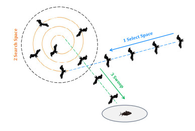
Three-dimensional path planning refers to determining an optimal path in a three-dimensional space with obstacles, so that the path is as close to the target location as possible, while meeting some other constraints, including distance, altitude, threat area, flight time, energy consumption, and so on. Although the bald eagle search algorithm has the characteristics of simplicity, few control parameters, and strong global search capabilities, it has not yet been applied to complex three-dimensional path planning problems. In order to broaden the application scenarios and scope of the algorithm and solve the path planning problem in three-dimensional space, we present a study where five three-dimensional geographical environments are simulated to represent real-life unmanned aerial vehicles flying scenarios. These maps effectively test the algorithm's ability to handle various terrains, including extreme environments. The experimental results have verified the excellent performance of the BES algorithm, which can quickly, stably, and effectively solve complex three-dimensional path planning problems, making it highly competitive in this field.
Citation: Yunhui Zhang, Yongquan Zhou, Shuangxi Chen, Wenhong Xiao, Mingyu Wu. Bald eagle search algorithm for solving a three-dimensional path planning problem[J]. Mathematical Biosciences and Engineering, 2024, 21(2): 2856-2878. doi: 10.3934/mbe.2024127
Three-dimensional path planning refers to determining an optimal path in a three-dimensional space with obstacles, so that the path is as close to the target location as possible, while meeting some other constraints, including distance, altitude, threat area, flight time, energy consumption, and so on. Although the bald eagle search algorithm has the characteristics of simplicity, few control parameters, and strong global search capabilities, it has not yet been applied to complex three-dimensional path planning problems. In order to broaden the application scenarios and scope of the algorithm and solve the path planning problem in three-dimensional space, we present a study where five three-dimensional geographical environments are simulated to represent real-life unmanned aerial vehicles flying scenarios. These maps effectively test the algorithm's ability to handle various terrains, including extreme environments. The experimental results have verified the excellent performance of the BES algorithm, which can quickly, stably, and effectively solve complex three-dimensional path planning problems, making it highly competitive in this field.

| [1] | J. B. Hiriart-Urruty, W. Oettli, J. Stoer, Optimization: Theory and Algorithms, CRC Press, 2020. https://doi.org/10.1201/9781003065098 |
| [2] | M. Tyagi, A. Sachdeva, V. Sharma, Optimization Methods in Engineering, Springer, 2021. https://doi.org/10.1007/978-981-15-4550-4 |
| [3] | P. Adby, Introduction to Optimization Methods, Springer Science & Business Media, 2013. |
| [4] | A. P. Engelbrecht, Computational Intelligence: An Introduction, John Wiley & Sons, 2007. https://doi.org/10.1002/9780470512517 |
| [5] |
J. S. Raj, A comprehensive survey on the computational intelligence techniques and its applications, J. ISMAC, 01 (2019), 147–159. https://doi.org/10.36548/jismac.2019.3.002 doi: 10.36548/jismac.2019.3.002

|
| [6] |
K. Hussain, M. N. Mohd Salleh, S. Cheng, Y. Shi, Metaheuristic research: a comprehensive survey, Artif. Intell. Rev., 52 (2019), 2191–2233. https://doi.org/10.1007/s10462-017-9605-z doi: 10.1007/s10462-017-9605-z
|
| [7] |
S. Yin, Q. Luo, Y. Zhou, EOSMA: An equilibrium optimizer slime mould algorithm for engineering design problems, Arab. J. Sci. Eng., 47 (2022), 10115–10146. https://doi.org/10.1007/s13369-021-06513-7 doi: 10.1007/s13369-021-06513-7
|
| [8] |
Y. Zhang, Y. Zhou, G. Zhou, Q. Luo, B. Zhu, A curve approximation approach using bio-inspired polar coordinate bald eagle search algorithm, Int. J. Comput. Intell. Sys., 15 (2022), 30. https://doi.org/10.1007/s44196-022-00084-7 doi: 10.1007/s44196-022-00084-7
|
| [9] |
N. Du, Y. Zhou, W. Deng, Q. Luo, Improved chimp optimization algorithm for three-dimensional path planning problem, Mul. Tools Appl., 81 (2022), 27397–27422. https://doi.org/10.1007/s11042-022-12882-4 doi: 10.1007/s11042-022-12882-4
|
| [10] |
M. Kumar, M. Husain, N. Upreti, D. Gupta, Genetic algorithm: Review and application, J. SSRN Elec., 2010 (2010). https://doi.org/10.2139/ssrn.3529843 doi: 10.2139/ssrn.3529843
|
| [11] |
R. Storn, K. Price, Differential evolution–A simple and efficient heuristic for global optimization over continuous spaces, J. Global Optim., 11 (1997), 341–359. https://doi.org/10.1023/A:1008202821328 doi: 10.1023/A:1008202821328
|
| [12] | J. Kennedy, R. Eberhart, Particle swarm optimization, in Proceedings of ICNN'95–International Conference on Neural Networks, (1995), 1942–1948. |
| [13] |
M. Dorigo, V. Maniezzo, A. Colorni, Ant system: optimization by a colony of cooperating agents, IEEE Trans. Syst. Man Cybern. Part B, 26 (1996), 29–41. https://doi.org/10.1109/3477.484436 doi: 10.1109/3477.484436
|
| [14] |
S. Mirjalili, A. Lewis, The whale optimization algorithm, Adv. Eng. Software, 95 (2016), 51–67. https://doi.org/10.1016/j.advengsoft.2016.01.008 doi: 10.1016/j.advengsoft.2016.01.008
|
| [15] |
X. S. Yang, S. Deb, Cuckoo search: recent advances and applications, Neural Comput. Appl., 24 (2014), 169–174. https://doi.org/10.1007/s00521-013-1367-1 doi: 10.1007/s00521-013-1367-1
|
| [16] |
S. Li, H. Chen, M. Wang, A. A. Heidari, S. Mirjalili, Slime mould algorithm: A new method for stochastic optimization, Future Gener. Comput. Syst., 111 (2020), 300–323. https://doi.org/10.1016/j.future.2020.03.055 doi: 10.1016/j.future.2020.03.055
|
| [17] |
A. Faramarzi, M. Heidarinejad, S. Mirjalili, A. H. Gandomi, Marine predators algorithm: A nature-inspired metaheuristic, Exp. Syst. Appl., 152 (2020), 113377. https://doi.org/10.1016/j.eswa.2020.113377 doi: 10.1016/j.eswa.2020.113377
|
| [18] |
B. Abdollahzadeh, F. S. Gharehchopogh, S. Mirjalili, African vultures optimization algorithm: A new nature-inspired metaheuristic algorithm for global optimization problems, Comput. Ind. Eng., 158 (2021), 107408. https://doi.org/10.1016/j.cie.2021.107408 doi: 10.1016/j.cie.2021.107408
|
| [19] |
H. A. Alsattar, A. A. Zaidan, B. B. Zaidan, Novel meta-heuristic bald eagle search optimisation algorithm, Artif. Intell. Rev., 53 (2020), 2237–2264. https://doi.org/10.1007/s10462-019-09732-5 doi: 10.1007/s10462-019-09732-5
|
| [20] | D. Huang, X. Zhu, A novel method based on chemical reaction optimization for pairwise sequence alignment, in Parallel Computational Fluid Dynamics, Springer Berlin Heidelberg, (2014), 429–439. https://doi.org/10.1007/978-3-642-53962-6_38 |
| [21] |
F. A. Hashim, K. Hussain, E. H. Houssein, M. S. Mabrouk, W. Al-Atabany, Archimedes optimization algorithm: a new metaheuristic algorithm for solving optimization problems, Appl. Intell., 51 (2021), 1531–1551. https://doi.org/10.1007/s10489-020-01893-z doi: 10.1007/s10489-020-01893-z
|
| [22] |
A. Rabehi, B. Nail, H. Helal, A. Douara, A. Ziane, M. Amrani, et al., Optimal estimation of Schottky diode parameters using a novel optimization algorithm: Equilibrium optimizer, Superlattices Microstruct., 146 (2020), 106665. https://doi.org/10.1016/j.spmi.2020.106665 doi: 10.1016/j.spmi.2020.106665
|
| [23] |
R. V. Rao, V. J. Savsani, D. P. Vakharia, Teaching–learning-based optimization: A novel method for constrained mechanical design optimization problems, Comput. Aided Des., 43 (2011), 303–315. https://doi.org/10.1016/j.cad.2010.12.015 doi: 10.1016/j.cad.2010.12.015
|
| [24] |
A. W. Mohamed, A. A. Hadi, A. K. Mohamed, Gaining-sharing knowledge based algorithm for solving optimization problems: a novel nature-inspired algorithm, Int. J. Mach. Learn. Cybern., 11 (2020), 1501–1529. https://doi.org/10.1007/s13042-019-01053-x doi: 10.1007/s13042-019-01053-x
|
| [25] |
Y. B. Chen, Y. S., Mei, J. Q. Yu, X. L. Su, N. Xu, Three-dimensional unmanned aerial vehicle path planning using modified wolf pack search algorithm, Neurocomputing, 266 (2017), 445–457. https://doi.org/10.1016/j.neucom.2017.05.059 doi: 10.1016/j.neucom.2017.05.059
|
| [26] |
H. Duan, Y. Yu, X. Zhang, S. Shao, Three-dimension path planning for UCAV using hybrid meta-heuristic ACO-DE algorithm, Simul. Modell. Pract. Theory, 18 (2010), 1104–1115. https://doi.org/10.1016/j.simpat.2009.10.006 doi: 10.1016/j.simpat.2009.10.006
|
| [27] |
P. Saxena, S. Tayal, R. Gupta, A. Maheshwari, G. Kaushal, R. Tiwari, Three dimensional route planning for multiple unmanned aerial vehicles using salp swarm algorithm, J. Exp. Theor. Artif. Intell., 35 (2023), 1059–1078. https://doi.org/10.1080/0952813X.2022.2059107 doi: 10.1080/0952813X.2022.2059107
|
| [28] |
U. Goel, S. Varshney, A. Jain, S. Maheshwari, A. Shukla, Three dimensional path planning for UAVs in dynamic environment using glow-worm swarm optimization, Proc. Comput. Sci., 133 (2018), 230–239. https://doi.org/10.1016/j.procs.2018.07.028 doi: 10.1016/j.procs.2018.07.028
|
| [29] |
Y. Zhang, Y. Zhou, G. Zhou, Q. Luo, An effective multi-objective bald eagle search algorithm for solving engineering design problems, Appl. Soft Comput., 145 (2023), 110585. https://doi.org/10.1016/j.asoc.2023.110585 doi: 10.1016/j.asoc.2023.110585
|
| [30] |
S. Yin, Q. Luo, Y. Zhou, IBMSMA: An indicator-based multi-swarm slime mould algorithm for multi-objective truss optimization problems, J. Bionic Eng., 20 (2023), 1333–1360. https://doi.org/10.1007/s42235-022-00307-9 doi: 10.1007/s42235-022-00307-9
|
| [31] |
G. I. Sayed, M. M. Soliman, A. E. Hassanien, A novel melanoma prediction model for imbalanced data using optimized SqueezeNet by bald eagle search optimization, Comput. Bio. Med., 136 (2021), 104712. https://doi.org/10.1016/j.compbiomed.2021.104712 doi: 10.1016/j.compbiomed.2021.104712
|
| [32] |
H. A. Almashhadani, X. Deng, S. N. A. Latif, M. M. Ibrahim, O. H. R. Al-hwaidi, Deploying an efficient and reliable scheduling for mobile edge computing for IoT applications, Mater. Today Proc., 80 (2023), 2850–2857. https://doi.org/10.1016/j.matpr.2021.07.050 doi: 10.1016/j.matpr.2021.07.050
|
| [33] |
A. M. Nassef, A. Fathy, H. Rezk, D. Yousri, Optimal parameter identification of supercapacitor model using bald eagle search optimization algorithm, J. Energy Storage, 50 (2022), 104603. https://doi.org/10.1016/j.est.2022.104603 doi: 10.1016/j.est.2022.104603
|
| [34] |
A. D. Algarni, N. Alturki, N. F. Soliman, S. Abdel-Khalek, A. A. A. Mousa, An improved bald eagle search algorithm with deep learning model for forest fire detection using hyperspectral remote sensing images, Can. J. Remote Sens, 48 (2022), 609–620. https://doi.org/10.1080/07038992.2022.2077709 doi: 10.1080/07038992.2022.2077709
|
| [35] |
A. Eid, S. Kamel, H. M. Zawbaa, M. Dardeer, Improvement of active distribution systems with high penetration capacities of shunt reactive compensators and distributed generators using bald eagle search, Ain Shams Eng. J., 13 (2022), 101792. https://doi.org/10.1016/j.asej.2022.101792 doi: 10.1016/j.asej.2022.101792
|
| [36] |
S. Alsubai, M. Hamdi, S. Abdel-Khalek, A. Alqahtani, A. Binbusayyis, R. F. Mansour, Bald eagle search optimization with deep transfer learning enabled age-invariant face recognition model, Image Vis. Comput., 126 (2022), 104545. https://doi.org/10.1016/j.imavis.2022.104545 doi: 10.1016/j.imavis.2022.104545
|
| [37] |
M. Elsisi, M. E. S. M. Essa, Improved bald eagle search algorithm with dimension learning-based hunting for autonomous vehicle including vision dynamics, Appl. Intell., 53 (2023), 11997–12014. https://doi.org/10.1007/s10489-022-04059-1 doi: 10.1007/s10489-022-04059-1
|
| [38] |
Y. Chen, W. Wu, P. Jiang, C. Wan, An improved bald eagle search algorithm for global path planning of unmanned vessel in complicated waterways, J. Mar. Sci. Eng., 11 (2023), 118. https://doi.org/10.3390/jmse11010118 doi: 10.3390/jmse11010118
|
| [39] |
S. Dian, J. Zhong, B. Guo, J. Liu, R. Guo, A smooth path planning method for mobile robot using a BES-incorporated modified QPSO algorithm, Expert Syst. Appl., 208 (2022), 118256. https://doi.org/10.1016/j.eswa.2022.118256 doi: 10.1016/j.eswa.2022.118256
|
| [40] |
Y. Niu, X. Yan, Y. Wang, Y. Niu, Three-dimensional collaborative path planning for multiple UCAVs based on improved artificial ecosystem optimizer and reinforcement learning, Knowl. Based Syst., 276 (2023), 110782. https://doi.org/10.1016/j.knosys.2023.110782 doi: 10.1016/j.knosys.2023.110782
|
| [41] |
G. Hu, B. Du, G. Wei, HG-SMA: hierarchical guided slime mould algorithm for smooth path planning, Artif. Intell. Rev., 56 (2023), 9267–9327. https://doi.org/10.1007/s10462-023-10398-3 doi: 10.1007/s10462-023-10398-3
|
| [42] |
D. Agarwal, P. S. Bharti, Implementing modified swarm intelligence algorithm based on Slime moulds for path planning and obstacle avoidance problem in mobile robots, Appl. Soft Comput., 107 (2021), 107372. https://doi.org/10.1016/j.asoc.2021.107372 doi: 10.1016/j.asoc.2021.107372
|
| [43] |
Y. Cui, W. Hu, A. Rahmani, Multi-robot path planning using learning-based artificial bee colony algorithm, Eng. Appl. Artif. Intell., 129 (2024), 107579. https://doi.org/10.1016/j.engappai.2023.107579 doi: 10.1016/j.engappai.2023.107579
|
| [44] |
C. Miao, G. Chen, C. Yan, Y. Wu, Path planning optimization of indoor mobile robot based on adaptive ant colony algorithm, Comput. Ind. Eng., 156 (2021), 107230. https://doi.org/10.1016/j.cie.2021.107230 doi: 10.1016/j.cie.2021.107230
|
| [45] |
X. Yu, C. Li, J. Zhou, A constrained differential evolution algorithm to solve UAV path planning in disaster scenarios, Knowl. Based Syst., 204 (2020), 106209. https://doi.org/10.1016/j.knosys.2020.106209 doi: 10.1016/j.knosys.2020.106209
|
| [46] |
R. Wang, M. Lungu, Z. Zhou, X. Zhu, Y. Ding, Q. Zhao, Least global position information based control of fixed-wing UAVs formation flight: Flight tests and experimental validation, Aerosp. Sci. Technol., 140 (2023), 108473. https://doi.org/10.1016/j.ast.2023.108473 doi: 10.1016/j.ast.2023.108473
|
| [47] |
P. C. Song, J. S. Pan, S. C. Chu, A parallel compact cuckoo search algorithm for three-dimensional path planning, Appl. Soft Comput., 94 (2020), 106443. https://doi.org/10.1016/j.asoc.2020.106443 doi: 10.1016/j.asoc.2020.106443
|
| [48] | T. Ren, R. Zhou, J. Xia, Z. Dong, Three-dimensional path planning of UAV based on an improved A* algorithm, in 2016 IEEE Chinese Guidance, Navigation and Control Conference (CGNCC), (2016), 140–145. https://doi.org/10.1109/CGNCC.2016.7828772 |
| [49] | H. Daryanavard, A. Harifi, UAV path planning for data gathering of IoT nodes: ant colony or simulated annealing optimization, in 2019 3rd International Conference on Internet of Things and Applications (IoT), (2019), 1–4. https://doi.org/10.1109/IICITA.2019.8808834 |
| [50] | Q. Wang, A. Zhang, L. Qi, Three-dimensional path planning for UAV based on improved PSO algorithm, in the 26th Chinese Control and Decision Conference (2014 CCDC), (2014), 3981–3985. https://doi.org/10.1109/CCDC.2014.6852877 |
| [51] |
C. Qu, W. Gai, J. Zhang, M. Zhong, A novel hybrid grey wolf optimizer algorithm for unmanned aerial vehicle (UAV) path planning, Knowl. Based Syst., 194 (2020), 105530. https://doi.org/10.1016/j.knosys.2020.105530 doi: 10.1016/j.knosys.2020.105530
|
| [52] | U. Cekmez, M. Ozsiginan, O. K. Sahingoz, A UAV path planning with parallel ACO algorithm on CUDA platform, in 2014 International Conference on Unmanned Aircraft Systems (ICUAS), (2014), 347–354. https://doi.org/10.1109/ICUAS.2014.6842273 |
| [53] | S. Ghambari, L. Idoumghar, L. Jourdan, J. Lepagnot, An improved TLBO algorithm for solving UAV path planning problem, in 2019 IEEE Symposium Series on Computational Intelligence (SSCI), IEEE, (2019), 2261–2268. https://doi.org/10.1109/SSCI44817.2019.9003160 |
| [54] | S. Ghambari, J. Lepagnot, L. Jourdan, L. Idoumghar, A comparative study of meta-heuristic algorithms for solving UAV path planning, in 2018 IEEE Symposium Series on Computational Intelligence (SSCI), (2018), 174–181. https://doi.org/10.1109/SSCI.2018.8628807 |
| [55] |
S. Zhang, Y. Zhou, Z. Li, W. Pan, Grey wolf optimizer for unmanned combat aerial vehicle path planning, Adv. Eng. Software, 99 (2016), 121–136. https://doi.org/10.1016/j.advengsoft.2016.05.015 doi: 10.1016/j.advengsoft.2016.05.015
|
| [56] |
S. Yin, Q. Luo, Y. Du, Y. Zhou, DTSMA: Dominant swarm with adaptive T-distribution mutation-based slime mould algorithm, Math. Biosci. Eng., 19 (2022), 2240–2285. https://doi.org/10.3934/mbe.2022105 doi: 10.3934/mbe.2022105
|
| [57] |
C. J. M. Moctezuma, J. Mora, M. G. Mendoza, A self-adaptive mechanism using weibull probability distribution to improve metaheuristic algorithms to solve combinatorial optimization problems in dynamic environments, Math. Biosci. Eng., 17 (2020), 975–997. https://doi.org/10.3934/mbe.2020052 doi: 10.3934/mbe.2020052
|
| [58] |
G. Zhou, Y. Zhou, W. Deng, S. Yin, Y. Zhang, Advances in teaching–learning-based optimization algorithm: A comprehensive survey (ICIC2022), Neurocomputing, 561 (2023), 126898. https://doi.org/10.1016/j.neucom.2023.126898 doi: 10.1016/j.neucom.2023.126898
|
| [59] |
A. E. Ezugwu, A. M. Ikotun, O. O. Oyelade, L. Abualigah, J. O. Agushaka, C. I. Eke, et al., A comprehensive survey of clustering algorithms: State-of-the-art machine learning applications, taxonomy, challenges, and future research prospects, Eng. Appl. Artif. Intell., 110 (2022), 104743. https://doi.org/10.1016/j.engappai.2022.104743 doi: 10.1016/j.engappai.2022.104743
|
| [60] |
P. Singh, N. Mittal, An efficient localization approach to locate sensor nodes in 3D wireless sensor networks using adaptive flower pollination algorithm, Wireless Networks, 27 (2021), 1999–2014. https://doi.org/10.1007/s11276-021-02557-7 doi: 10.1007/s11276-021-02557-7
|
| [61] |
K. Hu, L. Wang, J. Cai, L. Cheng, An improved genetic algorithm with dynamic neighborhood search for job shop scheduling problem, Math. Biosci. Eng., 20 (2023), 17407–17427. https://doi.org/10.3934/mbe.2023774 doi: 10.3934/mbe.2023774
|
| [62] |
T. Zhang, Y. Zhou, G. Zhou, W. Deng, Q. Luo, Discrete Mayfly Algorithm for spherical asymmetric traveling salesman problem, Exp. Syst. Appl., 221 (2023), 119765. https://doi.org/10.1016/j.eswa.2023.119765 doi: 10.1016/j.eswa.2023.119765
|


Figures(14) / Tables(5)

Yunhui Zhang, Yongquan Zhou, Shuangxi Chen, Wenhong Xiao, Mingyu Wu. Bald eagle search algorithm for solving a three-dimensional path planning problem[J]. Mathematical Biosciences and Engineering, 2024, 21(2): 2856-2878. doi: 10.3934/mbe.2024127


 DownLoad: