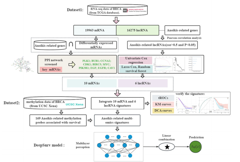
As a type of programmed cell death, anoikis resistance plays an essential role in tumor metastasis, allowing cancer cells to survive in the systemic circulation and as a key pathway for regulating critical biological processes. We conducted an exploratory analysis to improve risk stratification and optimize adjuvant treatment choices for patients with breast cancer, and identify multigene features in mRNA and lncRNA transcriptome profiles associated with anoikis. First, the variance selection method filters low information content genes in RNA sequence and then extracts the mRNA and lncRNA expression data base on annotation files. Then, the top ten key mRNAs are screened out through the PPI network. Pearson analysis has been employed to identify lncRNAs related to anoikis, and the prognosis-related lncRNAs are selected using Univariate Cox regression and machine learning. Finally, we identified a group of RNAs (including ten mRNAs and six lncRNAs) and integrated the expression data of 16 genes to construct a risk-scoring system for BRCA prognosis and drug sensitivity analysis. The risk score's validity has been evaluated with the ROC curve, Kaplan-Meier survival curve analysis and decision curve analysis (DCA). For the methylation data, we have obtained 169 anoikis-related prognostic methylation sites, integrated these sites with 16 RNA features and further used the deep learning model to evaluate and predict the survival risk of patients. The developed anoikis feature is demonstrated a consistency index (C-index) of 0.778, indicating its potential to predict the survival probability of breast cancer patients using deep learning methods.
Citation: Huili Yang, Wangren Qiu, Zi Liu. Anoikis-related mRNA-lncRNA and DNA methylation profiles for overall survival prediction in breast cancer patients[J]. Mathematical Biosciences and Engineering, 2024, 21(1): 1590-1609. doi: 10.3934/mbe.2024069
As a type of programmed cell death, anoikis resistance plays an essential role in tumor metastasis, allowing cancer cells to survive in the systemic circulation and as a key pathway for regulating critical biological processes. We conducted an exploratory analysis to improve risk stratification and optimize adjuvant treatment choices for patients with breast cancer, and identify multigene features in mRNA and lncRNA transcriptome profiles associated with anoikis. First, the variance selection method filters low information content genes in RNA sequence and then extracts the mRNA and lncRNA expression data base on annotation files. Then, the top ten key mRNAs are screened out through the PPI network. Pearson analysis has been employed to identify lncRNAs related to anoikis, and the prognosis-related lncRNAs are selected using Univariate Cox regression and machine learning. Finally, we identified a group of RNAs (including ten mRNAs and six lncRNAs) and integrated the expression data of 16 genes to construct a risk-scoring system for BRCA prognosis and drug sensitivity analysis. The risk score's validity has been evaluated with the ROC curve, Kaplan-Meier survival curve analysis and decision curve analysis (DCA). For the methylation data, we have obtained 169 anoikis-related prognostic methylation sites, integrated these sites with 16 RNA features and further used the deep learning model to evaluate and predict the survival risk of patients. The developed anoikis feature is demonstrated a consistency index (C-index) of 0.778, indicating its potential to predict the survival probability of breast cancer patients using deep learning methods.

| [1] | Y. S. Sun, Z. Zhao, Z. N. Yang, F. Xu, H. J. Lu, Z. Y. Zhu, et al., Risk factors and preventions of breast cancer, Int. J. Biol. Sci., 13 (2017), 1387–1397. https://doi.org/10.7150%2Fijbs.21635 |
| [2] |
T. J. Key, P. K. Verkasalo, E. Banks, Epidemiology of breast cancer, Lancet Oncol., 2 (2001), 133–140. https://doi.org/10.1016/S1470-2045(00)00254-0 doi: 10.1016/S1470-2045(00)00254-0

|
| [3] |
Y. N. Kim, K. H. Koo, J. Y. Sung, U. J. Yun, H. Kim, Anoikis resistance: an essential prerequisite for tumor metastasis, Int. J. Cell Biol., 2012 (2012), e306879. https://doi.org/10.1155/2012/306879 doi: 10.1155/2012/306879
|
| [4] |
S. Frisch, H. Francis, Disruption of epithelial cell-matrix interactions induces apoptosis, J. Cell Biol., 124 (1994), 619–626. https://doi.org/10.1083/jcb.124.4.619 doi: 10.1083/jcb.124.4.619
|
| [5] |
M. C. Guadamillas, A. Cerezo, M. A. del Pozo, Overcoming anoikis–pathways to anchorage-independent growth in cancer, J. Cell Sci., 124 (2011), 3189–3197. https://doi.org/10.1242/jcs.072165 doi: 10.1242/jcs.072165
|
| [6] |
Y. Luo, W. Q. Tang, S. S. Xiang, J. B. Feng, X. Y. Zu, Non-coding RNAs in breast cancer: Implications for programmed cell death, Cancer Lett., 550 (2022), 215929. https://doi.org/10.1016/j.canlet.2022.215929 doi: 10.1016/j.canlet.2022.215929
|
| [7] |
D. Fanfone, Z. C. Wu, J. Mammi, K. Berthenet, D. Neves, K. Weber, et al., Confined migration promotes cancer metastasis through resistance to anoikis and increased invasiveness, eLife, 11 (2022), e73150. https://doi.org/10.7554/eLife.73150 doi: 10.7554/eLife.73150
|
| [8] |
K. Zhao, Z. Wang, T. Hackert, C. Pitzer, M. Zöller, Tspan8 and Tspan8/CD151 knockout mice unravel the contribution of tumor and host exosomes to tumor progression, J. Exp. Clin. Cancer Res., 37 (2018), 312. https://doi.org/10.1186/s13046-018-0961-6 doi: 10.1186/s13046-018-0961-6
|
| [9] |
C. Akekawatchai, S. Roytrakul, S. Kittisenachai, P. Isarankura-Na-Ayudhya, S. Jitrapakdee, Protein profiles associated with anoikis resistance of metastatic MDA-MB-231 breast cancer cells, Asian Pac. J. Cancer Prev., 17 (2016), 581–590. https://doi.org/10.7314/APJCP.2016.17.2.581 doi: 10.7314/APJCP.2016.17.2.581
|
| [10] |
B. Weigelt, J. L. Peterse, L. J. van't Veer, Breast cancer metastasis: markers and models, Nat. Rev. Cancer, 5 (2005), 591–602. https://doi.org/10.1038/nrc1670 doi: 10.1038/nrc1670
|
| [11] |
W. Q. Li, J. Lee, H. G. Vikis, S. H. Lee, G. F. Liu, J. Aurandt, et al., Activation of FAK and Src are receptor-proximal events required for netrin signaling, Nat. Neurosci., 7 (2004), 1213–1221. https://doi.org/10.1038/nn1329 doi: 10.1038/nn1329
|
| [12] |
Y. Su, H. J. Wu, A. Pavlosky, L. L. Zou, X. N. Deng, Z. X. Zhang, et al., Regulatory non-coding RNA: new instruments in the orchestration of cell death, Cell Death Dis., 7 (2016), e2333. https://doi.org/10.1038/cddis.2016.210 doi: 10.1038/cddis.2016.210
|
| [13] |
M. Rebhan, V. Chalifa-Caspi, J. Prilusky, D. Lance, GeneCards: integrating information about genes, proteins and diseases, Trends Genet., 13 (1997), 163. https://doi.org/10.1016/s0168-9525(97)01103-7 doi: 10.1016/s0168-9525(97)01103-7
|
| [14] |
M. E. Ritchie, B. Phipson, D. Wu, Y. F. Hu, C. W. Law, W. Shi, et al., Limma powers differential expression analyses for RNA-sequencing and microarray studies, Nucleic Acids Res., 43 (2015), e47. https://doi.org/10.1093/nar/gkv007 doi: 10.1093/nar/gkv007
|
| [15] |
H. V. Cook, N.T. Doncheva, D. Szklarczyk, C. von Mering, J. L. Juhl, STRING: A virus-host protein-protein interaction database, Viruses, 10 (2018), 519. https://doi.org/10.3390/v10100519 doi: 10.3390/v10100519
|
| [16] |
P. Shannon, A. Markiel, O. Ozier, N. S. Baliga, J. T. Wang, D. Ramage, et al., Cytoscape: A software environment for integrated models of biomolecular interaction networks, Genome Res., 13 (2003), 2498–2504. http://www.genome.org/cgi/doi/10.1101/gr.1239303 doi: 10.1101/gr.1239303
|
| [17] |
C. H. Chin, S. H. Chen, H. H. Wu, C. W. Ho, M. T. Ko, C. Y. Lin, cytoHubba: identifying hub objects and sub-networks from complex interactome, BMC Syst. Biol., 8 (2014), S11. https://doi.org/10.1186/1752-0509-8-S4-S11 doi: 10.1186/1752-0509-8-S4-S11
|
| [18] |
D. R. Cox, Regression models and life-tables, J. R. Stat. Soc. B., 34 (1972), 187–202. https://doi.org/10.1111/j.2517-6161.1972.tb00899.x doi: 10.1111/j.2517-6161.1972.tb00899.x
|
| [19] |
R. Tibshirani, The lasso method for variable selection in the Cox model, Stat. Med., 16 (1997), 385–395. https://doi.org/10.1002/(SICI)1097-0258(19970228)16:4<385::AID-SIM380>3.0.CO;2-3 doi: 10.1002/(SICI)1097-0258(19970228)16:4<385::AID-SIM380>3.0.CO;2-3
|
| [20] | N. Simon, J. Friedman, T. Hastie, R. Tibshirani, Regularization paths for Cox's proportional hazards model via coordinate descent, J. Stat. Software, 39 (2011), 1–13. https://doi.org/10.18637%2Fjss.v039.i05 |
| [21] |
H. Ishwaran, U. B. Kogalur, E. H. Blackstone, M. S. Lauer, Random survival forests, Ann. Appl. Stat., 2 (2008), 841–860. https://doi.org/10.1214/08-AOAS169 doi: 10.1214/08-AOAS169
|
| [22] |
X. Chen, H. Ishwaran, Random forests for genomic data analysis, Genomics, 99 (2012), 323–329. https://doi.org/10.1016/j.ygeno.2012.04.003 doi: 10.1016/j.ygeno.2012.04.003
|
| [23] |
H. Q. Lin, D. Zelterman, Modeling survival data: extending the Cox model, Technometrics, 44 (2002), 85–86. https://doi.org/10.1198/tech.2002.s656 doi: 10.1198/tech.2002.s656
|
| [24] |
A. N. Kamarudin, T. Cox, R. Kolamunnage-Dona, Time-dependent ROC curve analysis in medical research: current methods and applications, BMC Med. Res. Methodol., 17 (2017), 53. https://doi.org/10.1186/s12874-017-0332-6 doi: 10.1186/s12874-017-0332-6
|
| [25] |
S. Monti, P. Tamayo, J. Mesirov, T. Golub, Consensus clustering: a resampling-based method for class discovery and visualization of gene expression microarray data, Mach. Learn., 52 (2003), 91–118. https://doi.org/10.1023/A:1023949509487 doi: 10.1023/A:1023949509487
|
| [26] |
W. J. Yang, J. Soares, P. Greninger, E. J. Edelman, H. Lightfoot, S. Forbes, et al., Genomics of Drug Sensitivity in Cancer (GDSC): a resource for therapeutic biomarker discovery in cancer cells, Nucleic Acids Res., 41 (2013), D955–D961. https://doi.org/10.1093/nar/gks1111 doi: 10.1093/nar/gks1111
|
| [27] |
D. Maeser, R. F. Gruener, R. S. Huang, OncoPredict: an R package for predicting in vivo or cancer patient drug response and biomarkers from cell line screening data, Briefings Bioinf., 22 (2021), bbab260. https://doi.org/10.1093/bib/bbab260 doi: 10.1093/bib/bbab260
|
| [28] |
J. L. Katzman, U. Shaham, A. Cloninger, J. Bates, T. Jiang, Y. Kluger, DeepSurv: personalized treatment recommender system using a Cox proportional hazards deep neural network, BMC Med. Res. Methodol., 18 (2018), 1–12. https://doi.org/10.1186/s12874-018-0482-112 doi: 10.1186/s12874-018-0482-112
|
| [29] |
J. Adeoye, L. L. Hui, M. Koohi-Moghadam, J. Y. Tan, S. W. Choi, P. Thomson, Comparison of time-to-event machine learning models in predicting oral cavity cancer prognosis, Int. J. Med. Inf., 157 (2022), 104635. https://doi.org/10.1016/j.ijmedinf.2021.104635 doi: 10.1016/j.ijmedinf.2021.104635
|
| [30] | F. Zhu, R. Zhong, F. Li, C. C. Li, N. Din, H. Sweidan, et al., Development and validation of a deep transfer learning-based multivariable survival model to predict overall survival in lung cancer, Transl. Lung Cancer Res., 12 (2023), 471–482. https://doi.org/10.21037%2Ftlcr-23-84 |
| [31] |
B. Lausen, M. Schumacher, Maximally selected rank statistics, Biometrics, 48 (1992), 73–85. https://doi.org/10.2307/2532740 doi: 10.2307/2532740
|
| [32] |
I. Bichindaritz, G. H. Liu, C. Bartlett, Integrative survival analysis of breast cancer with gene expression and DNA methylation data, Bioinformatics, 37 (2021), 2601–2608. https://doi.org/10.1093/bioinformatics/btab140 doi: 10.1093/bioinformatics/btab140
|
| [33] |
J. Cheng, J. Zhang, Y. Han, X. S. Wang, X. F. Ye, Y. B. Meng, et al., Integrative analysis of histopathological images and genomic data predicts clear cell renal cell carcinoma prognosis, Cancer Res., 77 (2017), e91–e100. https://doi.org/10.1158/0008-5472.CAN-17-0313 doi: 10.1158/0008-5472.CAN-17-0313
|
| [34] |
Z. Y. Zhang, H. Chai, Y. Wang, Z. X. Pan, Y. D. Yang, Cancer survival prognosis with deep bayesian perturbation Cox network, Comput. Biol. Med., 141 (2022), 105012. https://doi.org/10.1016/j.compbiomed.2021.105012 doi: 10.1016/j.compbiomed.2021.105012
|
| [35] |
E. Kakavandi, R. Shahbahrami, H. Goudarzi, G. Eslami, E. Faghihloo, Anoikis resistance and oncoviruses, J. Cell. Biochem., 119 (2018), 2484–2491. https://doi.org/10.1002/jcb.26363 doi: 10.1002/jcb.26363
|
| [36] |
M. J. Zou, E. Y. Baitei, R. A. Al-Rijjal, R. S. Parhar, F. A. Al-Mohanna, S. Kimura, et al., KRASG12D-mediated oncogenic transformation of thyroid follicular cells requires long-term TSH stimulation and is regulated by SPRY1, Lab. Invest., 95 (2015), 1269–1277. https://doi.org/10.1038/labinvest.2015.90 doi: 10.1038/labinvest.2015.90
|
| [37] |
S. Li, Y. Chen, Y. H. Zhang, X. M. Jiang, Y. Jiang, X. Qin, et al., Shear stress promotes anoikis resistance of cancer cells via caveolin-1-dependent extrinsic and intrinsic apoptotic pathways, J. Cell. Physiol., 234 (2019), 3730–3743. https://doi.org/10.1002/jcp.27149 doi: 10.1002/jcp.27149
|
| [38] |
P. Chanvorachote, U. Nimmannit, Y. Lu, S. Talbott, B. H. Jiang, Y. Rojanasakul, Nitric oxide regulates lung carcinoma cell anoikis through inhibition of ubiquitin-proteasomal degradation of caveolin-1, J. Biol. Chem., 284 (2009), 28476–28484. https://doi.org/10.1074/jbc.M109.050864 doi: 10.1074/jbc.M109.050864
|
| [39] |
W. T. Chiu, H. T. Lee, F. J. Huang, K. D. Aldape, J. Yao, P. S. Steeg, et al., Caveolin-1 upregulation mediates suppression of primary breast tumor growth and brain metastases by stat3 inhibition, Cancer Res., 71 (2011), 4932–4943. https://doi.org/10.1158/0008-5472.CAN-10-4249 doi: 10.1158/0008-5472.CAN-10-4249
|
| [40] |
K. Strebhardt, A. Ullrich, Targeting polo-like kinase 1 for cancer therapy, Nat. Rev. Cancer, 6 (2006), 321–330. https://doi.org/10.1038/nrc1841 doi: 10.1038/nrc1841
|
| [41] |
R. M. Golsteyn, K. E. Mundt, A. M. Fry, E. A. Nigg, Cell cycle regulation of the activity and subcellular localization of Plk1, a human protein kinase implicated in mitotic spindle function, J. Cell Biol., 129 (1995), 1617–1628. https://doi.org/10.1083/jcb.129.6.1617 doi: 10.1083/jcb.129.6.1617
|
| [42] |
F. Toyoshima-Morimoto, E. Taniguchi, N. Shinya, A. Iwamatsu, E. Nishida, Polo-like kinase 1 phosphorylates cyclin B1 and targets it to the nucleus during prophase, Nature, 410 (2001), 215–220. https://doi.org/10.1038/35065617 doi: 10.1038/35065617
|
| [43] |
N. E. Bhola, V. M. Jansen, S. Bafna, J. M. Giltnane, J. M. Balko, M. V. Estrada, et al., Kinome-wide functional screen identifies role of PLK1 in hormone-independent, ER-positive breast cancer, Cancer Res., 75 (2015), 405–414. https://doi.org/10.1158/0008-5472.CAN-14-2475 doi: 10.1158/0008-5472.CAN-14-2475
|
| [44] |
A. P. Baron, C. Schubert, F. Cubizolles, G. Siemeister, M. Hitchcock, A. Mengel, et al., Probing the catalytic functions of Bub1 kinase using the small molecule inhibitors BAY-320 and BAY-524, Elife, 5 (2016), e12187. https://doi.org/10.7554/eLife.12187 doi: 10.7554/eLife.12187
|
| [45] |
B. Yuan, Y. Xu, J. H. Woo, Y. Y. Wang, Y. K. Bae, D. S. Yoon, et al., Increased expression of mitotic checkpoint genes in breast cancer cells with chromosomal instability, Clin. Cancer Res., 12 (2006), 405–410. https://doi.org/10.1158/1078-0432.CCR-05-0903 doi: 10.1158/1078-0432.CCR-05-0903
|
| [46] |
K. A. Myrie, M. J. Percy, J. N. Azim, C. K. Neeley, E. M. Petty, Mutation and expression analysis of human BUB1 and BUB1B in aneuploid breast cancer cell lines, Cancer Lett., 152 (2000), 193–199. https://doi.org/10.1016/S0304-3835(00)00340-2 doi: 10.1016/S0304-3835(00)00340-2
|
| [47] |
M. Uhlen, P. Oksvold, L. Fagerberg, E. Lundberg, K. Jonasson, M. Forsberg, et al., Towards a knowledge-based human protein atlas, Nat. Biotechnol., 28 (2010), 1248–1250. https://doi.org/10.1038/nbt1210-1248 doi: 10.1038/nbt1210-1248
|
| [48] |
Q. Shi, Z. Zhou, N. S. Ye, Q. L. Chen, X. X. Zheng, M. S. Fang, MiR-181a inhibits non-small cell lung cancer cell proliferation by targeting CDK1, Cancer Biomarkers, 20 (2017), 539–546. https://doi.org/10.3233/cbm-170350 doi: 10.3233/cbm-170350
|
| [49] |
C. V. Dang, K. A. O'Donnell, L. I. Zeller, T. Nguyen, R. C. Osthus, F. Li, The c-Myc target gene network, Semin. Cancer Biol., 16 (2006), 253–264. https://doi.org/10.1016/j.semcancer.2006.07.014 doi: 10.1016/j.semcancer.2006.07.014
|
| [50] |
A. N. Shajahan-Haq, K. L. Cook, J. L. Schwartz-Roberts, A. E. Eltayeb, D. M. Demas, A. M. Warri, et al., MYC regulates the unfolded protein response and glucose and glutamine uptake in endocrine resistant breast cancer, Mol. Cancer, 13 (2014), 239. https://doi.org/10.1186/1476-4598-13-239 doi: 10.1186/1476-4598-13-239
|
| [51] |
C. M. McNeil, C. M. Sergio, L. R. Anderson, C. K. Inman, S. A. Eggleton, N. C. Murphy, et al., c-Myc overexpression and endocrine resistance in breast cancer, J. Steroid Biochem. Mol. Biol., 102 (2006), 147–155. https://doi.org/10.1016/j.jsbmb.2006.09.028 doi: 10.1016/j.jsbmb.2006.09.028
|
| [52] |
S. Tsutsui, S. Ohno, S. Murakami, Y. Hachitanda, S. Oda, Prognostic value of epidermal growth factor receptor (EGFR) and its relationship to the estrogen receptor status in 1029 patients with breast cancer, Breast Cancer Res. Treat., 71 (2002), 67–75. https://doi.org/10.1023/A:1013397232011 doi: 10.1023/A:1013397232011
|
| [53] |
C. J. Witton, J. R. Reeves, J. J. Going, T. G. Cooke, J. M. Bartlett, Expression of the HER1–4 family of receptor tyrosine kinases in breast cancer, J. Pathol., 200 (2003), 290–297. https://doi.org/10.1002/path.1370 doi: 10.1002/path.1370
|
| [54] | R. W. Turkington, Stimulation of mammary carcinoma cell proliferation by epithelial growth factor in vitro1, Cancer Res., 29 (1969), 1457–1458. |
| [55] |
J. Taylor-Papadimitriou, M. Shearer, M. G. P. Stoker, Growth requirements of human mammary epithelial cells in culture, Int. J. Cancer, 20 (1977), 903–908. https://doi.org/10.1002/ijc.2910200613 doi: 10.1002/ijc.2910200613
|
| [56] |
M. G. P. Stoker, D. Pigott, J. Taylor-Papadimitriou, Response to epidermal growth factors of cultured human mammary epithelial cells from benign tumours, Nature, 264 (1976), 764–767. https://doi.org/10.1038/264764a0 doi: 10.1038/264764a0
|


Figures(11) / Tables(1)

Huili Yang, Wangren Qiu, Zi Liu. Anoikis-related mRNA-lncRNA and DNA methylation profiles for overall survival prediction in breast cancer patients[J]. Mathematical Biosciences and Engineering, 2024, 21(1): 1590-1609. doi: 10.3934/mbe.2024069


 DownLoad: