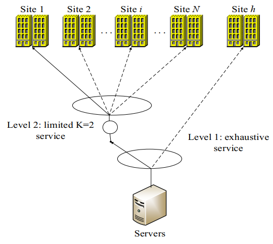
A continuous-time exhaustive-limited (K = 2) two-level polling control system is proposed to address the needs of increasing network scale, service volume and network performance prediction in the Internet of Things (IoT) and the Long Short-Term Memory (LSTM) network and an attention mechanism is used for its predictive analysis. First, the central site uses the exhaustive service policy and the common site uses the Limited K = 2 service policy to establish a continuous-time exhaustive-limited (K = 2) two-level polling control system. Second, the exact expressions for the average queue length, average delay and cycle period are derived using probability generating functions and Markov chains and the MATLAB simulation experiment. Finally, the LSTM neural network and an attention mechanism model is constructed for prediction. The experimental results show that the theoretical and simulated values basically match, verifying the rationality of the theoretical analysis. Not only does it differentiate priorities to ensure that the central site receives a quality service and to ensure fairness to the common site, but it also improves performance by 7.3 and 12.2%, respectively, compared with the one-level exhaustive service and the one-level limited K = 2 service; compared with the two-level gated- exhaustive service model, the central site length and delay of this model are smaller than the length and delay of the gated- exhaustive service, indicating a higher priority for this model. Compared with the exhaustive-limited K = 1 two-level model, it increases the number of information packets sent at once and has better latency performance, providing a stable and reliable guarantee for wireless network services with high latency requirements. Following on from this, a fast evaluation method is proposed: Neural network prediction, which can accurately predict system performance as the system size increases and simplify calculations.
Citation: Zhijun Yang, Wenjie Huang, Hongwei Ding, Zheng Guan, Zongshan Wang. Performance analysis of a two-level polling control system based on LSTM and attention mechanism for wireless sensor networks[J]. Mathematical Biosciences and Engineering, 2023, 20(11): 20155-20187. doi: 10.3934/mbe.2023893
A continuous-time exhaustive-limited (K = 2) two-level polling control system is proposed to address the needs of increasing network scale, service volume and network performance prediction in the Internet of Things (IoT) and the Long Short-Term Memory (LSTM) network and an attention mechanism is used for its predictive analysis. First, the central site uses the exhaustive service policy and the common site uses the Limited K = 2 service policy to establish a continuous-time exhaustive-limited (K = 2) two-level polling control system. Second, the exact expressions for the average queue length, average delay and cycle period are derived using probability generating functions and Markov chains and the MATLAB simulation experiment. Finally, the LSTM neural network and an attention mechanism model is constructed for prediction. The experimental results show that the theoretical and simulated values basically match, verifying the rationality of the theoretical analysis. Not only does it differentiate priorities to ensure that the central site receives a quality service and to ensure fairness to the common site, but it also improves performance by 7.3 and 12.2%, respectively, compared with the one-level exhaustive service and the one-level limited K = 2 service; compared with the two-level gated- exhaustive service model, the central site length and delay of this model are smaller than the length and delay of the gated- exhaustive service, indicating a higher priority for this model. Compared with the exhaustive-limited K = 1 two-level model, it increases the number of information packets sent at once and has better latency performance, providing a stable and reliable guarantee for wireless network services with high latency requirements. Following on from this, a fast evaluation method is proposed: Neural network prediction, which can accurately predict system performance as the system size increases and simplify calculations.

| [1] |
X. M. Wang, L. J. Du, Y. Zhang, X. Z. Zhao, X. Z. Cheng, Y. L. Tao, Priority queue-based polling mechanism on seismic equipment cluster monitoring, Cluster Comput., 20 (2017), 611–619. https://doi.org/10.1007/s10586-017-0726-6 doi: 10.1007/s10586-017-0726-6

|
| [2] |
G. Sudha, C. Tharini, Trust-based clustering and best route selection strategy for energy efficient wireless sensor networks, Automatika, 64 (2023), 634–641. https://doi.org/10.1080/00051144.2023.2208462 doi: 10.1080/00051144.2023.2208462
|
| [3] |
O. V. Semenova, D. T. Bui, The software package and its application to study the polling systems, Vestn. Tomsk. Gos. Univ. Upr. Vychislitelnaja Teh. Inform., 50 (2020), 106–113. https://doi.org/10.17223/19988605/50/13 doi: 10.17223/19988605/50/13
|
| [4] |
J. Y. Cao, W. X. Xie, Stability of a two-queue cyclic polling system with BMAPs under gated service and state-dependent time limited services disciplines, Queueing Syst., 85 (2017), 117–147. https://doi.org/10.1007/s11134-016-9504-z doi: 10.1007/s11134-016-9504-z
|
| [5] |
Z. Yang, Y. Sun, J. Gan, New polling scheme based on busy/idle queues mechanism, Int. J. Perform. Eng., 14 (2018), 2522–2531. https://doi.org/10.23940/ijpe.18.10.p28.25222531 doi: 10.23940/ijpe.18.10.p28.25222531
|
| [6] |
Y. X. Lv, Z. X. Liu, M. H. Bi, C. Hao, Y. R. Zhai, Selective polling and controlled contention based WLAN MAC scheme for low-latency applications, IEEE Commun. Lett., 27 (2023), 1050–1054. https://doi.org/10.1109/LCOMM.2023.3240191 doi: 10.1109/LCOMM.2023.3240191
|
| [7] |
B. R. Sathishkumar, An effectual spectrum sharing and battery utilization strategy using fuzzy enabled dynamic relay polling transmission in WSN, J. Intell. Fuzzy Syst., 44 (2023), 4907–4930. https://doi.org/10.3233/JIFS-223001 doi: 10.3233/JIFS-223001
|
| [8] |
M. F. Li, C. C. Fang, H. W. Ferng, On-demand energy transfer and energy-aware polling-based MAC for wireless powered sensor networks, Sensors, 22 (2022), 2476. https://doi.org/10.3390/s22072476 doi: 10.3390/s22072476
|
| [9] |
S. Siddiqui, A. A. khan, S. Ghani, Achieving energy efficiency in wireless sensor networks using dynamic channel polling and packet concatenation, China Commun., 18 (2021), 249–270. https://doi.org/10.23919/JCC.2021.08.018 doi: 10.23919/JCC.2021.08.018
|
| [10] | Z. Yang, Y. Su, H. W. Ding, Analysis of two-level polling system characteristics of exhaustive service and asymmetrically gated service, Acta Automatica Sin., 44 (2018), 2228–2237. |
| [11] |
Z. J. Han, H. W. Ding, L. Y. Bao, Z. J. Yang, Q. L. Liu, Analysis of new multi-priority P-CSMA of non-persistent type random multiple access ad hoc network in MAC protocol analysis, Int. J. Commun. Netw. Distr. Syst., 25 (2020), 57–77. https://doi.org/10.1504/IJCNDS.2020.108163 doi: 10.1504/IJCNDS.2020.108163
|
| [12] |
Z. Yang, L. Zhu, H. Ding, Z. Guan, A Priority-based parallel schedule polling MAC for wireless sensor networks, J. Commun., 11 (2016), 792–797. https://doi.org/10.12720/jcm.11.8.792-797 doi: 10.12720/jcm.11.8.792-797
|
| [13] |
A. Mercian, E. I. Gurrola, F. Aurzada, M. P. McGarry, M. Reisslein, Upstream polling protocols for flow control in PON/xDSL hybrid access networks, IEEE Trans. Commun., 64 (2016), 2971–2984. https://doi.org/10.1109/TCOMM.2016.2576450 doi: 10.1109/TCOMM.2016.2576450
|
| [14] |
H. Ding, C. Li, L. Bao, Z. Yang, L. Li, Q. Liu, Research on multi-level priority polling MAC protocol in FPGA tactical data chain, IEEE Access, 7 (2019), 33506–33516. https://doi.org/10.1109/ACCESS.2019.2902488 doi: 10.1109/ACCESS.2019.2902488
|
| [15] |
Z. Guan, Z. J. Yang, M. He, W. H. Qian, Analysis of time-delay characteristics of two-level polling control system relying on station states, J. Autom., 42 (2016), 1207–1214. https://doi.org/10.16383/j.aas.2016.c150226 doi: 10.16383/j.aas.2016.c150226
|
| [16] |
T. Jiang, X. Lu, L. Liu, J. Lv, X. Chai, Strategic behavior of customers and optimal control for batch service polling systems with priorities, Complexity, 2020 (2020). https://doi.org/10.1155/2020/6015372 doi: 10.1155/2020/6015372
|
| [17] |
W. H. Mu, L. Y. Bao, H. W. Ding, Y. F. Zhao, An exact analysis of discrete time two-level priority polling system based on multi-times gated service policy, Acta Electron. Sinica, 46 (2018), 276–280. https://doi.org/10.3969/j.issn.0372-2112.2018.02.003 doi: 10.3969/j.issn.0372-2112.2018.02.003
|
| [18] | Z. J. Yang, L. Mao, H. W. Ding, Q. L. Kou, Research on two-level priority polling access control protocol based on continuous time, in 2020 IEEE 6th International Conference on Computer and Communications, (2020), 136–140. https://doi.org/10.1109/ICCC51575.2020.9345093 |
| [19] |
Z. J. Yang, Z. Liu, H. W. Ding, Research of continuous-time two-level polling system performance of exhaustive service and gated service, J. Comput. Appl., 39 (2019), 2019–2023. https://doi.org/10.11772/j.issn.1001-9081.2019010063 doi: 10.11772/j.issn.1001-9081.2019010063
|
| [20] |
R. Gupta, J. Gupta, Federated learning using game strategies: state-of-the art and future trends, Comput. Netw., 225 (2023), 109650. https://doi.org/10.1016/j.comnet.2023.109650 doi: 10.1016/j.comnet.2023.109650
|
| [21] |
P. Boobalan, S. P. Ramu, Q. V. Pham, K. Dev, S. Pandya, P. K. R. Maddikunta, et al., Fusion of federated learning and industrial Internet of Tings: A survey, Comput. Netw., 212 (2022), 109048. https://doi.org/10.1016/j.comnet.2022.109048 doi: 10.1016/j.comnet.2022.109048
|
| [22] |
I. Guarino, G. Aceto, D. Ciuonzo, A. Montieri, V. Persico, A. Pescapè, Contextual counters and multimodal Deep Learning for activity-level traffic classification of mobile communication apps during COVID-19 pandemic, Comput. Netw., 219 (2022), 109452. https://doi.org/10.1016/j.comnet.2022.109452 doi: 10.1016/j.comnet.2022.109452
|
| [23] |
J. Liu, Q. Wang, Y. Xu, AR-GAIL: adaptive routing protocol for FANETs using generative adversarial imitation learning, Comput. Netw., 218 (2022), 109382. https://doi.org/10.1016/j.comnet.2022.109382 doi: 10.1016/j.comnet.2022.109382
|
| [24] |
Y. H. Liu, X. Y. Zhang, W. Y. Liu, Y. Lin, F. Su, J. Cui, et al., Seismic vulnerability and risk assessment at the urban scale using support vector machine and GI science technology: a case study of the Lixia District in Jinan City, China, Geomat. Nat. Haz. Risk, 14 (2023), 1947–5705. https://doi.org/10.1080/19475705.2023.2173663 doi: 10.1080/19475705.2023.2173663
|
| [25] |
P. Bhatt, A. L. Maclean, Comparison of high-resolution NAIP and unmanned aerial vehicle (UAV) imagery for natural vegetation communities classification using machine learning approaches, Gisci. Remote Sens., 60 (2023), 2177448. https://doi.org/10.1080/15481603.2023.2177448 doi: 10.1080/15481603.2023.2177448
|
| [26] |
M. B. Haile, A. O. Salau, B. Enyew, A. J. Belay, Detection and classification of gastrointestinal disease using convolutional neural network and SVM, Cogent Eng., 9 (2022), 2084878. https://doi.org/10.1080/23311916.2022.2084878 doi: 10.1080/23311916.2022.2084878
|
| [27] |
Wang J., Zhao Y. L., Y. C. Fu, L. L. Xia, J. S. Chen, Improving LSMA for impervious surface estimation in an urban area, Eur. J. Remote Sens., 55 (2022), 37–51. https://doi.org/10.1080/22797254.2021.2018666 doi: 10.1080/22797254.2021.2018666
|
| [28] |
N. Ali, Z. Halim, S. F. Hussain, An artificial intelligence-based framework for data-driven categorization of computer scientists: a case study of world's Top 10 computing departments, Scientometrics, 128 (2022), 1513–1545. https://doi.org/10.1007/s11192-022-04627-9 doi: 10.1007/s11192-022-04627-9
|
| [29] |
B. Akyuz, S. Karatay, F. Erken, Comparison of the performance of the regression models in GPS-Total electron content prediction, Politeknik Dergisi, 26 (2022), 321–328. https://doi.org/10.2339/politeknik.1137658 doi: 10.2339/politeknik.1137658
|
| [30] |
X. Y. Li, X. S. Han, M. Yang, Day-Ahead optimal dispatch strategy for active distribution network based on improved deep reinforcement learning, IEEE Access, 10 (2022), 9357–9370. https://doi.org/10.1109/ACCESS.2022.3141824 doi: 10.1109/ACCESS.2022.3141824
|
| [31] |
S. Dudey, F. Olimov, M. A. Rafique, J. Kim, M. Jeon, Label-attention transformer with geometrically coherent objects for image captioning, Inform. Sci., 623 (2022), 812–831. https://doi.org/10.1016/j.ins.2022.12.018 doi: 10.1016/j.ins.2022.12.018
|
| [32] |
R. Inokuchi, M. Iwagami, Y. Sun, A. Sakamoto, N. Tamiya, Machine learning models predicting under-triage in telephone triage, Ann. Med., 54 (2022), 2990–2997. https://doi.org/10.1080/07853890.2022.2136402 doi: 10.1080/07853890.2022.2136402
|
| [33] |
S. Janizadeh, S. M. Bateni, C. Jun, J. Im, H. T. Pai, S. S. Band, et al., Combination four different ensemble algorithms with the generalized linear model (GLM) for predicting forest fire susceptibility, Geomat. Nat. Haz. Risk, 14 (2023), 2206512. https://doi.org/10.1080/19475705.2023.2206512 doi: 10.1080/19475705.2023.2206512
|
| [34] |
S. Latif, X. W. Fang, K. Arshid, A. Almuhaimeed, A. Imran, M. Alghamdi, Analysis of birth data using ensemble modeling techniques, Appl. Artif. Intell., 37 (2023), 2158273. https://doi.org/10.1080/08839514.2022.2158273 doi: 10.1080/08839514.2022.2158273
|
| [35] |
Y. W. Tang, F. Qiu, B. J. Wang, D. Wu, L. H. Jing, Z. C. Sun, A deep relearning method based on the recurrent neural network for land cover classification, Gisci. Remote Sens., 59 (2022), 1344–1366. https://doi.org/10.1080/15481603.2022.2115589 doi: 10.1080/15481603.2022.2115589
|
| [36] |
G. C. Habek, M. A. Tocoglu, A. Onan, Bi-directional CNN-RNN architecture with group-wise enhancement and attention mechanisms for cryptocurrency sentiment analysis, Appl. Artif. Intell., 36 (2022), 2145641. https://doi.org/10.1080/08839514.2022.2145641 doi: 10.1080/08839514.2022.2145641
|
| [37] |
L. Jin, S. Li, B. Hu, RNN models for dynamic matrix inversion: A control-theoretical perspective, IEEE Trans. Ind. Inform., 14 (2018), 189–199. https://doi.org/10.1109/TII.2017.2717079 doi: 10.1109/TII.2017.2717079
|
| [38] |
Y. S. Zhang, J. Zhang, Y. R. Jiang, G. J. Huang, R. Y. Chen, A text sentiment classification modeling method based on coordinated CNN-LSTM-Attention model, Chinese J. Electr., 28 (2019), 120–126. https://doi.org/10.1049/cje.2018.11.004 doi: 10.1049/cje.2018.11.004
|
| [39] |
D. Zhang, G. Lindholm, H. Ratnaweera, Use long short-term memory to enhance Internet of Things for combined sewer overflow monitoring, J. Hydrol., 556 (2018), 409–418. https://doi.org/10.1016/j.jhydrol.2017.11.018 doi: 10.1016/j.jhydrol.2017.11.018
|
| [40] |
Y. N. Zhou, S. Y. Wang, T. J. Wu, L. Feng, W. Wu, J. C. Luo, et al., For-backward LSTM-based missing data reconstruction for time-series Landsat images, Gisci. Remote Sens., 59 (2022), 410–430. https://doi.org/10.1080/15481603.2022.2031549 doi: 10.1080/15481603.2022.2031549
|
| [41] |
J. Sridhar, R. Gobinath, M. S. Kirgiz, Evaluation of artificial neural network predicted mechanical properties of jute and bamboo fiber reinforced concrete ALONG with silica fume, J. Nat. Fibers, 20 (2023), 2162186. https://doi.org/10.1080/15440478.2022.2162186 doi: 10.1080/15440478.2022.2162186
|
| [42] |
W. H. AlAlaween, O. A. Abueed, A. H. AlAlawin, O. H. Abdallah, N. T. Albashabsheh, E. S. AbdelAll, et al., Artificial neural networks for predicting the demand and price of the hybrid electric vehicle spare parts, Cogent Eng., 9 (2022), 2075075. https://doi.org/10.1080/23311916.2022.2075075 doi: 10.1080/23311916.2022.2075075
|
| [43] |
T. A. H. Alghamdi, O. T. E. Abdusalam, F. Anayi, M. Packianather, An artificial neural network based harmonic distortions estimator for grid-connected power converter-based applications, Ain Shams Eng. J., 14 (2022), 101916. https://doi.org/10.1016/j.asej.2022.101916 doi: 10.1016/j.asej.2022.101916
|
| [44] |
M. K. Wei, X. B. Hu, H. X. Yuan, Residual displacement estimation of the bilinear SDOF systems under the near-fault ground motions using the BP neural network, Adv. Struct. Eng., 25 (2021), 552–571. https://doi.org/10.1177/13694332211058530 doi: 10.1177/13694332211058530
|
| [45] |
H. X. Zhou, A. L. Che, X. H. Shuai, Y. Zhang, A spatial evaluation method for earthquake disaster using optimized BP neural network model, Geomat. Nat. Haz. Risk, 14 (2023), 1–26. https://doi.org/10.1080/19475705.2022.2160664 doi: 10.1080/19475705.2022.2160664
|
| [46] |
Z. B. Qiu, Z. J. Wu, Y. Song, Sphere gap breakdown voltage prediction based on ISSA optimized BP neural network and effective electric field feature set, IEE J. Trans. Electr., 18 (2022), 506–514. https://doi.org/10.1002/tee.23750 doi: 10.1002/tee.23750
|
| [47] |
J. W. Hou, Y. J. Wang, B. Hou, J. Zhou, Q. Tian, Spatial simulation and prediction of air temperature based on CNN-LSTM, Appl. Artif. Intell., 37 (2023), 2166235. https://doi.org/10.1080/08839514.2023.2166235 doi: 10.1080/08839514.2023.2166235
|
| [48] |
W. S. Zhang, W. W. Guo, X. Liu, Y. Liu, J. Zhou, B. Li, et al. LSTM-based analysis of industrial IoT equipment. IEEE Access, 6 (2018), 23551–23560. https://doi.org/10.1109/access.2018.2825538 doi: 10.1109/ACCESS.2018.2825538
|
| [49] |
X. B. Shu, L. Y. Zhang, Y. L. Sun, J. H. Tang, Host-parasite: Graph LSTM-in-LSTM for group activity recognition, IEEE Trans. Neural Netw. Learning Syst., 32 (2020), 663–674. https://doi.org/10.1109/TNNLS.2020.2978942 doi: 10.1109/TNNLS.2020.2978942
|
| [50] |
T. X. Shu, J. H. Chen, V. K. Bhargava, C. W. de Silva, An energy-efficient dual prediction scheme using LMS filter and LSTM in wireless sensor networks for environment monitoring, IEEE Int. Things J., 6 (2019), 6736–6747. https://doi.org/10.1109/JIOT.2019.2911295 doi: 10.1109/JIOT.2019.2911295
|
| [51] |
R. Okumura, K. Mizutani, H. Harada, Efficient polling communications for multi-hop networks based on receiver-initiated MAC protocol, Ieice Trans. Commun., E104-B (2021), 550–562. https://doi.org/10.1587/transcom.2020EBP3095 doi: 10.1587/transcom.2020EBP3095
|
| [52] |
J. L. Guo, F. F. Li, T. Wang, S. B. Zhang, Y. Q. Zhao, Parameter analysis and optimization of polling-based medium access control protocol for multi-sensor communication, Int. J. Distrib. Sens. Netw., 17 (2021). https://doi.org/10.1177/15501477211007412 doi: 10.1177/15501477211007412
|
| [53] |
J. K. van Ommeren, A. Al Hanbali, R. J. Boucherie, Analysis of polling models with a self-ruling server, Queueing Syst., 94 (2020), 77–107. https://doi.org/10.1007/s11134-019-09639-6 doi: 10.1007/s11134-019-09639-6
|
| [54] | Y. Y. Sun, Z. J. Yang, Analysis and research on polling system of wireless sensor network, Electr. Meas. Tech., 41 (2018), 100–104. |
| [55] |
Z. J. Yang, Q. L. Kou, H. W. Ding, BSCP-MAC: A blockchain-based synchronous control polling MAC protocol for wireless sensor networks, J. Electr. Eng. Technol., 18 (2023), 3799–3810. https://doi.org/10.1007/s42835-023-01440-z doi: 10.1007/s42835-023-01440-z
|
| [56] | J. Y. Ge, L. Y. Bao, H. W. Ding, X. Y. Ding, Performance analysis of the first-order characteristics of two-level priority polling system based on parallel gated and exhaustive services mode, in 2021 IEEE 4th International Conference on Electronic Information and Communication Technology (ICEICT), (2021), 10–13. https://doi.org/10.1109/ICEICT53123.2021.9531122 |
| [57] | Z. H. Liu, Y. J. Li, J. Q. Yao, Z. N. Cai, G. B. Han, X. Y. Xie, Ultra-short-term forecasting method of wind power based on W-BiLSTM, in 2021 IEEE 4th International Electrical and Energy Conference (CIEEC), (2021), 1–6. https://doi.org/10.1109/CIEEC50170.2021.9511041 |


Figures(23) / Tables(4)

Zhijun Yang, Wenjie Huang, Hongwei Ding, Zheng Guan, Zongshan Wang. Performance analysis of a two-level polling control system based on LSTM and attention mechanism for wireless sensor networks[J]. Mathematical Biosciences and Engineering, 2023, 20(11): 20155-20187. doi: 10.3934/mbe.2023893


 DownLoad: