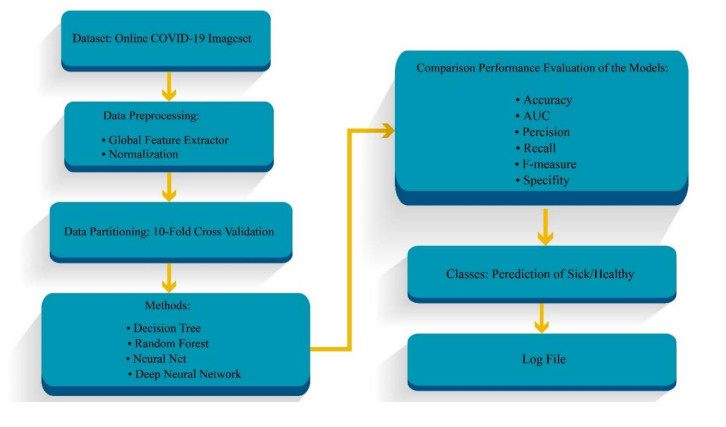
COVID-19 is most commonly diagnosed using a testing kit but chest X-rays and computed tomography (CT) scan images have a potential role in COVID-19 diagnosis. Currently, CT diagnosis systems based on Artificial intelligence (AI) models have been used in some countries. Previous research studies used complex neural networks, which led to difficulty in network training and high computation rates. Hence, in this study, we developed the 6-layer Deep Neural Network (DNN) model for COVID-19 diagnosis based on CT scan images. The proposed DNN model is generated to improve accurate diagnostics for classifying sick and healthy persons. Also, other classification models, such as decision trees, random forests and standard neural networks, have been investigated. One of the main contributions of this study is the use of the global feature extractor operator for feature extraction from the images. Furthermore, the 10-fold cross-validation technique is utilized for partitioning the data into training, testing and validation. During the DNN training, the model is generated without dropping out of neurons in the layers. The experimental results of the lightweight DNN model demonstrated that this model has the best accuracy of 96.71% compared to the previous classification models for COVID-19 diagnosis.
Citation: Javad Hassannataj Joloudari, Faezeh Azizi, Issa Nodehi, Mohammad Ali Nematollahi, Fateme Kamrannejhad, Edris Hassannatajjeloudari, Roohallah Alizadehsani, Sheikh Mohammed Shariful Islam. Developing a Deep Neural Network model for COVID-19 diagnosis based on CT scan images[J]. Mathematical Biosciences and Engineering, 2023, 20(9): 16236-16258. doi: 10.3934/mbe.2023725
COVID-19 is most commonly diagnosed using a testing kit but chest X-rays and computed tomography (CT) scan images have a potential role in COVID-19 diagnosis. Currently, CT diagnosis systems based on Artificial intelligence (AI) models have been used in some countries. Previous research studies used complex neural networks, which led to difficulty in network training and high computation rates. Hence, in this study, we developed the 6-layer Deep Neural Network (DNN) model for COVID-19 diagnosis based on CT scan images. The proposed DNN model is generated to improve accurate diagnostics for classifying sick and healthy persons. Also, other classification models, such as decision trees, random forests and standard neural networks, have been investigated. One of the main contributions of this study is the use of the global feature extractor operator for feature extraction from the images. Furthermore, the 10-fold cross-validation technique is utilized for partitioning the data into training, testing and validation. During the DNN training, the model is generated without dropping out of neurons in the layers. The experimental results of the lightweight DNN model demonstrated that this model has the best accuracy of 96.71% compared to the previous classification models for COVID-19 diagnosis.

| [1] |
F. Khozeimeh, D. Sharifrazi, N. H. Izadi, J. Hassannataj Joloudari, A. Shoeibi, R. Alizadehsani, et al., Combining a convolutional neural network with autoencoders to predict the survival chance of COVID-19 patients, Sci. Rep., 11 (2021), 1–18. https://doi.org/10.1038/s41598-021-93543-8 doi: 10.1038/s41598-021-93543-8

|
| [2] |
S. U. Kumar, D. T. Kumar, B. P. Christopher, C. Doss, The rise and impact of COVID-19 in India, Front. Med., 7 (2020), 250. https://doi.org/10.3389/fmed.2020.00250 doi: 10.3389/fmed.2020.00250
|
| [3] |
A. Guihur, M. E. Rebeaud, B. Fauvet, S. Tiwari, Y. G. Weiss, P. Goloubinoff, Moderate fever cycles as a potential mechanism to protect the respiratory system in COVID-19 patients, Front. Med., 7 (2020), 583. https://doi.org/10.3389/fmed.2020.564170 doi: 10.3389/fmed.2020.564170
|
| [4] |
R. J. Reiter, P. Abreu-Gonzalez, P. E. Marik, A. Dominguez-Rodriguez, Therapeutic algorithm for use of melatonin in patients with COVID-19, Front. Med., 7 (2020), 226. https://doi.org/10.3389/fmed.2020.00226 doi: 10.3389/fmed.2020.00226
|
| [5] |
M. R. Mahmoudi, D. Baleanu, S. S. Band, A. Mosavi, Factor analysis approach to classify COVID-19 datasets in several regions, Results Phys., 25 (2021), 104071. https://doi.org/10.1016/j.rinp.2021.104071 doi: 10.1016/j.rinp.2021.104071
|
| [6] |
N. Ayoobi, D. Sharifrazi, R. Alizadehsani, A. Shoeibi, J. M. Gorriz, H. Moosaei, et al., Time Series Forecasting of New Cases and New Deaths Rate for COVID-19 using Deep Learning Methods, Results Phys., 27 (2021), 104495. https://doi.org/10.1016/j.rinp.2021.104495 doi: 10.1016/j.rinp.2021.104495
|
| [7] |
A. Pak, O. A. Adegboye, A. I. Adekunle, K. M. Rahman, E. S. McBryde, D. P. Eisen, Economic consequences of the COVID-19 outbreak: the need for epidemic preparedness, Front. Public Health., 8 (2020), 241. https://doi.org/10.3389/fpubh.2020.00241 doi: 10.3389/fpubh.2020.00241
|
| [8] |
J. R. Larsen, M. R. Martin, J. D. Martin, P. Kuhn, J. B. Hicks, Modeling the onset of symptoms of COVID-19, Front. Public Health., 8 (2020), 473. https://doi.org/10.3389/fpubh.2020.00473 doi: 10.3389/fpubh.2020.00473
|
| [9] |
P. R. Bassi, R. Attux, A deep convolutional neural network for COVID-19 detection using chest X-rays, Res. Biomed. Eng., 38 (2021), 139–148. https://doi.org/10.1007/s42600-021-00132-9 doi: 10.1007/s42600-021-00132-9
|
| [10] |
Z. Nabizadeh-Shahre-Babak, N. Karimi, P. Khadivi, R. Roshandel, A. Emami, S. Samavi, Detection of COVID-19 in X-ray images by classification of bag of visual words using neural networks, Biomed. Signal Process. Control, 68 (2021), 102750. https://doi.org/10.1016/j.bspc.2021.102750 doi: 10.1016/j.bspc.2021.102750
|
| [11] | T. Zebin, S. Rezvy, COVID-19 detection and disease progression visualization: Deep learning on chest X-rays for classification and coarse localization, Appl. Intell., 51 (2021), 1010–1021. https://doi.org/10.1007%2Fs10489-020-01867-1 |
| [12] |
J. C. Gomes, A. I. Masood, L. H. de S. Silva, J. R. B. da Cruz Ferreira, A. A. Freire Junior, A. L. d. S. Rocha, et al., Covid-19 diagnosis by combining RT-PCR and pseudo-convolutional machines to characterize virus sequences, Sci. Rep., 11 (2021), 11545. https://doi.org/10.1038/s41598-021-90766-7 doi: 10.1038/s41598-021-90766-7
|
| [13] |
P. Bhardwaj, A. Kaur, A novel and efficient deep learning approach for COVID-19 detection using X-ray imaging modality, Int. J. Imaging Syst. Technol., 31 (2021), 1775–1791. https://doi.org/10.1002/ima.22627 doi: 10.1002/ima.22627
|
| [14] |
E. Hussain, M. Hasan, M. A. Rahman, I. Lee, T. Tamanna, M. Z. Parvez, CoroDet: A deep learning based classification for COVID-19 detection using chest X-ray images, Chaos Solit. Fractals, 142 (2021), 110495. https://doi.org/10.1016/j.chaos.2020.110495 doi: 10.1016/j.chaos.2020.110495
|
| [15] | H. Tabrizchi, A. Mosavi, Z. Vamossy, A. R. Varkonyi-Koczy, Densely Connected Convolutional Networks (DenseNet) for Diagnosing Coronavirus Disease (COVID-19) from Chest X-ray Imaging, in 2021 IEEE International Symposium on Medical Measurements and Applications (MeMeA), 2021, 1–5. https://doi.org/10.1109/MeMeA52024.2021.9478715 |
| [16] |
A. Scohy, A. Anantharajah, M. Bodéus, B. Kabamba-Mukadi, A. Verroken, H. Rodriguez-Villalobos, Low performance of rapid antigen detection test as frontline testing for COVID-19 diagnosis, J. Gen. Virol., 129 (2020), 104455. https://doi.org/10.1016/j.jcv.2020.104455 doi: 10.1016/j.jcv.2020.104455
|
| [17] |
R. M. Amer, M. Samir, O. A. Gaber, N. A. El-Deeb, A. A. Abdelmoaty, A. A. Ahmed, et al., Diagnostic performance of rapid antigen test for COVID-19 and the effect of viral load, sampling time, subject's clinical and laboratory parameters on test accuracy, J. Infect. Public Health, 14 (2021), 1446–1453. https://doi.org/10.1016/j.jiph.2021.06.002 doi: 10.1016/j.jiph.2021.06.002
|
| [18] |
J. Dinnes, P. Sharma, S. Berhane, S. S. van Wyk, N. Nyaaba, J. Domen, et al., Rapid, point-of-care antigen tests for diagnosis of SARS-CoV-2 infection, Cochrane Database Syst. Rev., 7 (2022). https://doi.org/10.1002/14651858.cd013705.pub3 doi: 10.1002/14651858.cd013705.pub3
|
| [19] | M. Berrimi, S. Hamdi, R. Y. Cherif, A. Moussaoui, M. Oussalah, M. Chabane, COVID-19 detection from Xray and CT scans using transfer learning, in 2021 International Conference of Women in Data Science at Taif University (WiDSTaif), 2021, 1–6. https://doi.org/10.1109/WiDSTaif52235.2021.9430229 |
| [20] |
V. Shah, R. Keniya, A. Shridharani, M. Punjabi, J. Shah, N. Mehendale, Diagnosis of COVID-19 using CT scan images and deep learning techniques, Emerg. Radiol., 28 (2021), 497–505. https://doi.org/10.1007/s10140-020-01886-y doi: 10.1007/s10140-020-01886-y
|
| [21] |
M. Singh, S. Bansal, S. Ahuja, R. K. Dubey, B. K. Panigrahi, N. Dey, Transfer learning–based ensemble support vector machine model for automated COVID-19 detection using lung computerized tomography scan data, Med. Biol. Eng. Comput., 59 (2021), 825–839. https://doi.org/10.1007/s11517-020-02299-2 doi: 10.1007/s11517-020-02299-2
|
| [22] |
R. L. Bard, Image-guided management of COVID-19 lung disease, Springer Nature, 2021. https://doi.org/10.1007/978-3-030-66614-9 doi: 10.1007/978-3-030-66614-9
|
| [23] |
G. Muhammad, M. S. Hossain, COVID-19 and non-COVID-19 classification using multi-layers fusion from lung ultrasound images, Inf. Fusion, 72 (2021), 80–88. https://doi.org/10.1016/j.inffus.2021.02.013 doi: 10.1016/j.inffus.2021.02.013
|
| [24] |
C.-C. Lai, T.-P. Shih, W.-C. Ko, H.-J. Tang, P.-R. Hsueh, Severe acute respiratory syndrome coronavirus 2 (SARS-CoV-2) and coronavirus disease-2019 (COVID-19): The epidemic and the challenges, Int. J. Antimicrob. Agents, 55 (2020), 105924. https://doi.org/10.1016/j.ijantimicag.2020.105924 doi: 10.1016/j.ijantimicag.2020.105924
|
| [25] |
F. Chua, D. Armstrong-James, S. R. Desai, J. Barnett, V. Kouranos, O. M. Kon, et al., The role of CT in case ascertainment and management of COVID-19 pneumonia in the UK: insights from high-incidence regions, Lancet Respir. Med., 8 (2020), 438–440. https://doi.org/10.1016/S2213-2600(20)30132-6 doi: 10.1016/S2213-2600(20)30132-6
|
| [26] |
Y. Fang, H. Zhang, J. Xie, M. Lin, L. Ying, P. Pang, et al., Sensitivity of chest CT for COVID-19: comparison to RT-PCR, Radiology, 296 (2020), E115–E117. https://doi.org/10.1148/radiol.2020200432 doi: 10.1148/radiol.2020200432
|
| [27] |
H. Abbasimehr, R. Paki, Prediction of COVID-19 confirmed cases combining deep learning methods and Bayesian optimization, Chaos Solit. Fractals, 142 (2021), 110511. https://doi.org/10.1016/j.chaos.2020.110511 doi: 10.1016/j.chaos.2020.110511
|
| [28] |
M. Zivkovic, N. Bacanin, K. Venkatachalam, A. Nayyar, A. Djordjevic, I. Strumberger, et al., COVID-19 cases prediction by using hybrid machine learning and beetle antennae search approach, Sustain. Cities Soc., 66 (2021), 102669. https://doi.org/10.1016/j.scs.2020.102669 doi: 10.1016/j.scs.2020.102669
|
| [29] |
S. Johri, M. Goyal, S. Jain, M. Baranwal, V. Kumar, R. Upadhyay, A novel machine learning-based analytical framework for automatic detection of COVID-19 using chest X-ray images, Int. J. Imaging Syst. Technol., 31 (2021), 1105–1119. https://doi.org/10.1002/ima.22613 doi: 10.1002/ima.22613
|
| [30] |
F. Falter, N. J. Screaton, Imaging the ICU Patient, Springer, 2014. https://doi.org/10.1007/978-0-85729-781-5 doi: 10.1007/978-0-85729-781-5
|
| [31] |
J. Musulin, S. Baressi Šegota, D. Štifanić, I. Lorencin, N. Anđelić, T. Šušteršič, et al., Application of Artificial Intelligence-Based Regression Methods in the Problem of COVID-19 Spread Prediction: A Systematic Review, Int. J. Environ, 18 (2021), 4287. https://doi.org/10.3390/ijerph18084287 doi: 10.3390/ijerph18084287
|
| [32] | P. K. Sethy, S. K. Behera, Detection of coronavirus disease (covid-19) based on deep features, 2020. https://doi.org/10.20944/preprints202003.0300.v1 |
| [33] |
A. M. Ismael, A. Şengür, Deep learning approaches for COVID-19 detection based on chest X-ray images, Expert Syst. Appl, 164 (2021), 114054. https://doi.org/10.1016/j.eswa.2020.114054 doi: 10.1016/j.eswa.2020.114054
|
| [34] |
A. I. Khan, J. L. Shah, M. M. Bhat, CoroNet: A deep neural network for detection and diagnosis of COVID-19 from chest x-ray images, Comput. Methods Programs Biomed., 196 (2020), 105581. https://doi.org/10.1016/j.cmpb.2020.105581 doi: 10.1016/j.cmpb.2020.105581
|
| [35] |
V. Shah, R. Keniya, A. Shridharani, M. Punjabi, J. Shah, N. Mehendale, Diagnosis of COVID-19 using CT scan images and deep learning techniques, Emerg. Radiol., 28 (2021), 497–505. https://doi.org/10.1007/s10140-020-01886-y doi: 10.1007/s10140-020-01886-y
|
| [36] |
M. Polsinelli, L. Cinque, G. Placidi, A light CNN for detecting COVID-19 from CT scans of the chest, Pattern Recognit. Lett., 140 (2020), 95–100. https://doi.org/10.1016/j.patrec.2020.10.001 doi: 10.1016/j.patrec.2020.10.001
|
| [37] |
S. A. Harmon, L. Cinque, G. Placidi, Artificial intelligence for the detection of COVID-19 pneumonia on chest CT using multinational datasets, Nat. Commun., 11 (2020), 1–7. https://doi.org/10.1016/j.patrec.2020.10.001 doi: 10.1016/j.patrec.2020.10.001
|
| [38] |
M. Loey, G. Manogaran, N. E. M. Khalifa, A deep transfer learning model with classical data augmentation and cgan to detect covid-19 from chest CT radiography digital images, Neural. Comput. Appl., 2020, 1–13. https://doi.org/10.1007/s00521-020-05437-x doi: 10.1007/s00521-020-05437-x
|
| [39] |
M. Singh, S. Bansal, S. Ahuja, R. K. Dubey, B. K. Panigrahi, N. Dey, Transfer learning–based ensemble support vector machine model for automated COVID-19 detection using lung computerized tomography scan data, Med. Biol. Eng. Comput., 59 (2021), 825–839. https://doi.org/10.1007/s11517-020-02299-2 doi: 10.1007/s11517-020-02299-2
|
| [40] |
M. Canayaz, S. Şehribanoğlu, R. Özdağ, M. Demir, COVID-19 diagnosis on CT images with Bayes optimization-based deep neural networks and machine learning algorithms, Neural. Comput. Appl., 34 (2022), 5349–5365. https://doi.org/10.1007/s00521-022-07052-4 doi: 10.1007/s00521-022-07052-4
|
| [41] |
M. Chieregato, F. Frangiamore, M. Morassi, C. Baresi, S. Nici, C. Bassetti, et al., A hybrid machine learning/deep learning COVID-19 severity predictive model from CT images and clinical data, Sci. Rep., 12 (2022), 1–15. https://doi.org/10.1038/s41598-022-07890-1 doi: 10.1038/s41598-022-07890-1
|
| [42] |
V. Ravi, H. Narasimhan, C. Chakraborty, T. D. Pham, Deep learning-based meta-classifier approach for COVID-19 classification using CT scan and chest X-ray images, Multimed. Syst., 28 (2022), 1401–1415. https://doi.org/10.1007/s00530-021-00826-1 doi: 10.1007/s00530-021-00826-1
|
| [43] |
Y. Liu, L. J. Durlofsky, 3D CNN-PCA: A deep-learning-based parameterization for complex geomodels, Comput. Geosci., 148 (2021), 104676. https://doi.org/10.1016/j.cageo.2020.104676 doi: 10.1016/j.cageo.2020.104676
|
| [44] |
S. Cheng, Y Jin, S. P. Harrison, C. Quilodrán-Casas, I. C. Prentice, Y. K. Guo, et al., Parameter flexible wildfire prediction using machine learning techniques: Forward and inverse modelling, Remote Sens., 14 (2022), 3228. https://doi.org/10.3390/rs14133228 doi: 10.3390/rs14133228
|
| [45] |
A. H. Barshooi, A. Amirkhani, A novel data augmentation based on Gabor filter and convolutional deep learning for improving the classification of COVID-19 chest X-Ray images, Biomed. Signal Process. Control., 72 (2022), 103326. https://doi.org/10.1016/j.bspc.2021.103326 doi: 10.1016/j.bspc.2021.103326
|
| [46] |
S. Aggarwal, S. Gupta, A. Alhudhaif, D. Koundal, R. Gupta, K. Polat, Automated COVID-19 detection in chest X-ray images using fine-tuned deep learning architectures, Expert Syst., 39 (2022), 1–17. https://doi.org/10.1111/exsy.12749 doi: 10.1111/exsy.12749
|
| [47] |
P. Nadler, S. Wang, R. Arcucci, X. Yang, Y. Guo, An epidemiological modelling approach for COVID-19 via data assimilation, Eur. J. Epidemiol., 35 (2020), 749–761. https://doi.org/10.1007/s10654-020-00676-7 doi: 10.1007/s10654-020-00676-7
|
| [48] |
L. Song, X. Liu, S. Chen, S. Liu, X. Liu, K. Muhammad, et al., A deep fuzzy model for diagnosis of COVID-19 from CT images, Appl. Soft Comput., 122 (2022), 108883. https://doi.org/10.1016/j.asoc.2022.108883 doi: 10.1016/j.asoc.2022.108883
|
| [49] |
C. Wen, S. Liu, S. Liu, A. A. Heidari, M. Hijji, C. Zarco, et al., ACSN: Attention capsule sampling network for diagnosing COVID-19 based on chest CT scans, Comput. Biol. Med., 153 (2023), 106338. https://doi.org/10.1016/j.compbiomed.2022.106338 doi: 10.1016/j.compbiomed.2022.106338
|
| [50] |
S. Cheng, C. C. Pain, Y.-K. Guo, R. Arcucci, Real-time updating of dynamic social networks for COVID-19 vaccination strategies, J. Ambient Intell. Humaniz Comput., 2023, 1–14. https://doi.org/10.1007/s12652-023-04589-7 doi: 10.1007/s12652-023-04589-7
|
| [51] |
J. Hodler, G. K. von Schulthess, C. L. Zollikofer, Diseases of the heart, chest & breast: diagnostic imaging and interventional techniques, Springer Science & Business Media, 2007. https://doi.org/10.1007/978-88-470-0633-1 doi: 10.1007/978-88-470-0633-1
|
| [52] |
M. M. Hefeda, CT chest findings in patients infected with COVID-19: Review of literature, Egypt. J. Radiol. Nucl. Med., 51 (2020), 1–15. https://doi.org/10.1186/s43055-020-00355-3 doi: 10.1186/s43055-020-00355-3
|
| [53] |
C. Bao, X. Liu, H. Zhang, Y. Li, J. Liu, Coronavirus disease 2019 (COVID-19) CT findings: A systematic review and meta-analysis, J. Am. Coll. Radiol., 17 (2020), 701–709. https://doi.org/10.1016/j.jacr.2020.03.006 doi: 10.1016/j.jacr.2020.03.006
|
| [54] | R. Kohavi, A study of cross-validation and bootstrap for accuracy estimation and model selection, in Proceedings of the 14th international joint conference on Artificial intelligence, 2 (1995), 1137–1143. https://doi.org/10.5555/1643031.1643047 |
| [55] |
J. Hassannataj Joloudari, F. Azizi, M. A. Nematollahi, R. Alizadehsani, E. Hassannatajjeloudari, I. Nodehi, et al., GSVMA: A Genetic Support Vector Machine ANOVA Method for CAD Diagnosis, Front. Cardiovasc. Med., 8 (2021), 760178. https://doi.org/10.3389/fcvm.2021.760178 doi: 10.3389/fcvm.2021.760178
|
| [56] |
J. Hassannataj Joloudari, M. Haderbadi, A. Mashmool, M. GhasemiGol, S. S. Band, A. Mosavi, Early detection of the advanced persistent threat attack using performance analysis of deep learning, IEEE Access, 8 (2020), 186125–186137. https://doi.org/10.1109/ACCESS.2020.3029202 doi: 10.1109/ACCESS.2020.3029202
|
| [57] |
J. Hassannataj Joloudari, E. Hassannataj Joloudari, H. Saadatfar, M. Ghasemigol, S. M. Razavi, A. Mosavi, et al., Coronary artery disease diagnosis; ranking the significant features using a random trees model, Int. J. Environ., 17 (2020), 731. https://doi.org/10.3390/ijerph17030731 doi: 10.3390/ijerph17030731
|
| [58] |
J. H. Joloudari, H. Saadatfar, A. Dehzangi, S. Shamshirband, Computer-aided decision-making for predicting liver disease using PSO-based optimized SVM with feature selection, Inform. Med. Unlocked, 17 (2019), 100255. https://doi.org/10.1016/j.imu.2019.100255 doi: 10.1016/j.imu.2019.100255
|
| [59] |
A. P. Bradley, The use of the area under the ROC curve in the evaluation of machine learning algorithms, Pattern Recognit., 30 (1997), 1145–1159. https://doi.org/10.1016/S0031-3203(96)00142-2 doi: 10.1016/S0031-3203(96)00142-2
|


Figures(15) / Tables(7)

Javad Hassannataj Joloudari, Faezeh Azizi, Issa Nodehi, Mohammad Ali Nematollahi, Fateme Kamrannejhad, Edris Hassannatajjeloudari, Roohallah Alizadehsani, Sheikh Mohammed Shariful Islam. Developing a Deep Neural Network model for COVID-19 diagnosis based on CT scan images[J]. Mathematical Biosciences and Engineering, 2023, 20(9): 16236-16258. doi: 10.3934/mbe.2023725


 DownLoad: