Effectively selecting discriminative brain regions in multi-modal neuroimages is one of the effective means to reveal the neuropathological mechanism of end-stage renal disease associated with mild cognitive impairment (ESRDaMCI). Existing multi-modal feature selection methods usually depend on the Euclidean distance to measure the similarity between data, which tends to ignore the implied data manifold. A self-expression topological manifold based multi-modal feature selection method (SETMFS) is proposed to address this issue employing self-expression topological manifold. First, a dynamic brain functional network is established using functional magnetic resonance imaging (fMRI), after which the betweenness centrality is extracted. The feature matrix of fMRI is constructed based on this centrality measure. Second, the feature matrix of arterial spin labeling (ASL) is constructed by extracting the cerebral blood flow (CBF). Then, the topological relationship matrices are constructed by calculating the topological relationship between each data point in the two feature matrices to measure the intrinsic similarity between the features, respectively. Subsequently, the graph regularization is utilized to embed the self-expression model into topological manifold learning to identify the linear self-expression of the features. Finally, the selected well-represented feature vectors are fed into a multicore support vector machine (MKSVM) for classification. The experimental results show that the classification performance of SETMFS is significantly superior to several state-of-the-art feature selection methods, especially its classification accuracy reaches 86.10%, which is at least 4.34% higher than other comparable methods. This method fully considers the topological correlation between the multi-modal features and provides a reference for ESRDaMCI auxiliary diagnosis.
Citation: Chaofan Song, Tongqiang Liu, Huan Wang, Haifeng Shi, Zhuqing Jiao. Multi-modal feature selection with self-expression topological manifold for end-stage renal disease associated with mild cognitive impairment[J]. Mathematical Biosciences and Engineering, 2023, 20(8): 14827-14845. doi: 10.3934/mbe.2023664
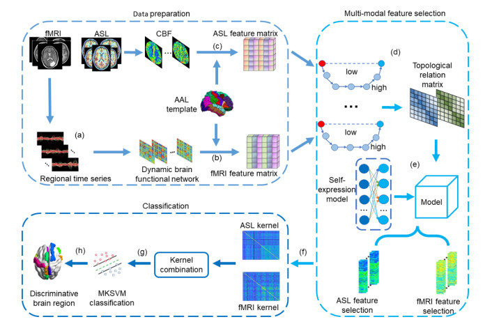
Effectively selecting discriminative brain regions in multi-modal neuroimages is one of the effective means to reveal the neuropathological mechanism of end-stage renal disease associated with mild cognitive impairment (ESRDaMCI). Existing multi-modal feature selection methods usually depend on the Euclidean distance to measure the similarity between data, which tends to ignore the implied data manifold. A self-expression topological manifold based multi-modal feature selection method (SETMFS) is proposed to address this issue employing self-expression topological manifold. First, a dynamic brain functional network is established using functional magnetic resonance imaging (fMRI), after which the betweenness centrality is extracted. The feature matrix of fMRI is constructed based on this centrality measure. Second, the feature matrix of arterial spin labeling (ASL) is constructed by extracting the cerebral blood flow (CBF). Then, the topological relationship matrices are constructed by calculating the topological relationship between each data point in the two feature matrices to measure the intrinsic similarity between the features, respectively. Subsequently, the graph regularization is utilized to embed the self-expression model into topological manifold learning to identify the linear self-expression of the features. Finally, the selected well-represented feature vectors are fed into a multicore support vector machine (MKSVM) for classification. The experimental results show that the classification performance of SETMFS is significantly superior to several state-of-the-art feature selection methods, especially its classification accuracy reaches 86.10%, which is at least 4.34% higher than other comparable methods. This method fully considers the topological correlation between the multi-modal features and provides a reference for ESRDaMCI auxiliary diagnosis.

| [1] |
L. Li, J. Y. Liu, F. X. Liang, H. D. Chen, R. G. Zhan, S. L. Zhao, et al., Altered brain function activity in patients with dysphagia after cerebral infarction: a resting-state functional magnetic resonance imaging study, Front. Neurol., 13 (2022), 782732. https://doi.org/10.3389/fneur.2022.782732 doi: 10.3389/fneur.2022.782732

|
| [2] |
S. H. Wang, Y. D. Zhang, G. Liu, P. Phillips, T. F. Yuan, Detection of Alzheimer's disease by three-dimensional displacement field estimation in structural magnetic resonance imaging, J. Alzheimer's Dis., 50 (2016), 233–248. https://doi.org/10.3233/JAD-150848 doi: 10.3233/JAD-150848
|
| [3] |
T. Tang, L. Huang, Y. S. Zhang, Z. F. Li, S. X. Liang, Aberrant pattern of regional cerebral blood flow in mild cognitive impairment: a meta-analysis of arterial spin labeling magnetic resonance imaging, Front. Aging Neurosci., 14 (2022), 961344. https://doi.org/10.3389/fnagi.2022.961344 doi: 10.3389/fnagi.2022.961344
|
| [4] |
J. X. Wang, S. C. Wu, Y. Sun, J. M. Lu, J. L. Zhang, Y. Fang, et al., Brain microstructural alterations in the left precuneus mediate the association between KIBRA polymorphism and working memory in healthy adults: a diffusion kurtosis imaging study, Brain Imaging Behav., 16 (2022), 2487–2496. https://doi.org/10.1007/s11682-022-00703-z doi: 10.1007/s11682-022-00703-z
|
| [5] |
Y. T. Zhang, Z. T. Xi, J. H. Zheng, H. F. Shi, Z. Q. Jiao, GWLS: A novel model for predicting cognitive function scores in patients with end-stage renal disease, Front. Aging Neurosci., 14 (2022), 834331. https://doi.org/10.3389/fnagi.2022.834331 doi: 10.3389/fnagi.2022.834331
|
| [6] |
Z. T. Xi, C. F. Song, J. H. Zheng, H. F. Shi, Z. Q. Jiao, Brain functional networks with dynamic hypergraph manifold regularization for classification of end-stage renal disease associated with mild cognitive impairment, CMES-Comp. Model. Eng. Sci., 135 (2023), 2243–2246. https://doi.org/10.32604/cmes.2023.023544 doi: 10.32604/cmes.2023.023544
|
| [7] |
Z. T. Xi, T. Q. Liu, H. F. Shi, Z. Q. Jiao, Hypergraph representation of multimodal brain networks for patients with end-stage renal disease associated with mild cognitive impairment, Math. Biosci. Eng., 20 (2023), 1882–1902. https://doi.org/10.3934/mbe.2023086 doi: 10.3934/mbe.2023086
|
| [8] |
Y. Li, J. Y. Liu, X. Q. Gao, B. Jie, K. Minjeong, Y. Pew-Thian, et al., Multimodal hyper-connectivity of functional networks using functionally-weighted LASSO for MCI classification, Med. Image Anal., 52 (2019), 80–96. https://doi.org/10.1016/j.media.2018.11.006 doi: 10.1016/j.media.2018.11.006
|
| [9] |
Z. Q. Jiao, S. W. Chen, H. F. Shi, J. Xu, Multi-modal feature selection with feature correlation and feature structure fusion for MCI and AD classification, Brain Sci., 12 (2022), 80. https://doi.org/10.3390/brainsci12010080 doi: 10.3390/brainsci12010080
|
| [10] |
X. Y. Liang, A. Connelly, F. Calamante, Graph analysis of resting-state ASL perfusion MRI data: Nonlinear correlations among CBF and network metrics, Neuroimage, 87 (2014), 265–275. https://doi.org/10.1016/j.neuroimage.2013.11.013 doi: 10.1016/j.neuroimage.2013.11.013
|
| [11] |
M. Havlicek, A. Roebroeck, K. Friston, A. Gardumi, D. Ivanov, K. Uludag, Physiologically informed dynamic causal modeling of fMRI data, Neuroimage, 122 (2015), 355–372. https://doi.org/10.1016/j.neuroimage.2015.07.078 doi: 10.1016/j.neuroimage.2015.07.078
|
| [12] |
D. C. Alsop, J. A. Detre, X. Golay, M. Gunther, J. Hendrikse, L. Hernandez-Garcia, et al., Recommended implementation of arterial spin-labeled perfusion MRI for clinical applications: a consensus of the ISMRM perfusion study group and the European consortium for ASL in dementia, Magn. Reason. Med., 73 (2015), 102–116. https://doi.org/10.1002/mrm.25197 doi: 10.1002/mrm.25197
|
| [13] | Y. Gao, C. Y. Wee, M. Kim, P. Giannakopoulos, M. L. Montandon, S. Haller, et al., MCI identification by joint learning on multiple MRI data, in Medical Image Computing and Computer-Assisted Intervention--MICCAI 2015: 18th International Conference, Springer, Munich, Germany, (2015), 78–85. https://doi.org/10.1007/978-3-319-24571-3_10 |
| [14] |
E. O'Lone, M. Connors, P. Masson, S. Wu, P. J. Kelly, D. Gillespie, et al., Cognition in people with end-stage kidney disease treated with hemodialysis: a systematic review and meta-analysis, Am. J. Kidney Dis., 67 (2016), 925–935. https://doi.org/10.1053/j.ajkd.2015.12.028 doi: 10.1053/j.ajkd.2015.12.028
|
| [15] |
J. M. Bugnicourt, O. Godefroy, J. M. Chillon, G. Choukroun, Z. A. Massy, Cognitive disorders and dementia in CKD: the neglected kidney-brain axis, J. Am. Soc. Nephrol., 24 (2013), 353–363. https://doi.org/10.1681/ASN.2012050536 doi: 10.1681/ASN.2012050536
|
| [16] |
Q. Z. Zeng, K. C. Li, X. Luo, S. Y. Wang, X. P. Xu, Z. Y. Li, Distinct atrophy pattern of hippocampal subfields in patients with progressive and stable mild cognitive impairment: A longitudinal MRI study, J. Alzheimer's Dis., 79 (2021), 237–247. https://doi.org/10.3233/JAD-200775 doi: 10.3233/JAD-200775
|
| [17] |
T. Iutaka, M. B. Freitas, S. S. Omar, F. A. Scortegagna, K. Nael, R. H. Nunes, et al., Arterial spin labeling: techniques, clinical applications, and interpretation, Radiographics, 43 (2023), e220088. https://doi.org/10.1148/rg.220088 doi: 10.1148/rg.220088
|
| [18] |
A. Camargo, Z. Wang, Hypo- and hyper-perfusion in MCI and AD identified by different ASL MRI sequences, Brain Imaging Behav., 17 (2023), 306–319. https://doi.org/10.1007/s11682-023-00764-8 doi: 10.1007/s11682-023-00764-8
|
| [19] |
Y. D. Zhang, S. H. Wang, Y. X. Sui, M. Yang, B. Liu, H. Cheng, et al., Multivariate approach for Alzheimer's disease detection using stationary wavelet entropy and predator-prey particle swarm optimization, J. Alzheimer's Dis., 65 (2018), 855–869. https://doi.org/10.3233/JAD-170069 doi: 10.3233/JAD-170069
|
| [20] |
W. M. Zheng, H. H. Liu, Z. G. Li, K. C. Li, Y. L. Wang, B. Hu, et al., Classification of Alzheimer's disease based on hippocampal multivariate morphometry statistics, CNS. Neurosci. Ther., 2023 (2023), 1–12. https://doi.org/10.1111/cns.14189 doi: 10.1111/cns.14189
|
| [21] |
B. Y. Lei, Y. Zhu, S. Z. Yu, H. Y. Hu, Y. W. Xu, G. H. Yue, Multi-scale enhanced graph convolutional network for mild cognitive impairment detection, Pattern Recognit., 134 (2023), 109106. https://doi.org/10.1016/j.patcog.2022.109106 doi: 10.1016/j.patcog.2022.109106
|
| [22] |
D. Q. Zhang, Y. P. Wang, L. P. Zhou, H. Yuan, D. G. Shen, Multimodal classification of Alzheimer's disease and mild cognitive impairment, Neuroimage, 55 (2011), 856–867. https://doi.org/10.1016/j.neuroimage.2011.01.008 doi: 10.1016/j.neuroimage.2011.01.008
|
| [23] |
B. Jie, D. Q. Zhang, B. Cheng, D. D. Shen, Manifold regularized multitask feature learning for multimodality disease classification, Hum. Brain Mapp., 36 (2015), 489–507. https://doi.org/10.1002/hbm.22642 doi: 10.1002/hbm.22642
|
| [24] |
Y. Shi, C. Zu, M. Hong, L. P. Zhou, L. Wang, X. Wu, et al., ASMFS: Adaptive-similarity-based multi-modality feature selection for classification of Alzheimer's disease, Pattern Recognit., 126 (2022), 108566. https://doi.org/10.1016/j.patcog.2022.108566 doi: 10.1016/j.patcog.2022.108566
|
| [25] | C. Y. Xu, C. C. Chen, Q. W. Guo, Y. W. Lin, X. Y. Meng, G. Z. Qiu, et al., A comparative study on the identification of amnestic mild cognitive impairment with MOCA-B and MES scales in China, J. Alzheimer's Dis. Relat. Disord., 4 (2021), 33–36. |
| [26] |
X. W. Song, Z. Y. Dong, X. Y. Long, S. F. Li, X. N. Zuo, C. Z. Zhu, et al., REST: A toolkit for resting-state functional magnetic resonance imaging data processing, PLoS One, 6 (2011), e25031. https://doi.org/10.1371/journal.pone.0025031 doi: 10.1371/journal.pone.0025031
|
| [27] |
C. G. Yan, Y. F. Zang, DPARSF: A MATLAB toolbox for "pipeline" data analysis of resting-state fMRI, Front. Syst. Neurosci., 14 (2010), 4–13. https://doi.org/10.3389/fnsys.2010.00013 doi: 10.3389/fnsys.2010.00013
|
| [28] | Q. Wang, M. Chen, X. L. Li, Quantifying and detecting collective motion by manifold learning, in 2017 AAAI Conference on Artificial Intelligence, AAAI, San Francisco, USA, (2017), 4292–4298. https://doi.org/10.1609/aaai.v31i1.11209 |
| [29] |
S. D. Huang, I. W. Tsang, Z. L. Xu, J. C. Lv, Measuring diversity in graph learning: A unified framework for structured multi-view clustering, IEEE Trans. Knowl. Data Eng., 34 (2022), 5869–5883. https://doi.org/10.1109/TKDE.2021.3068461 doi: 10.1109/TKDE.2021.3068461
|
| [30] |
D. P. Bertsekas, Nonlinear programming, J. Oper. Res. Soc., 48 (1997), 334. https://doi.org/10.1057/palgrave.jors.2600425 doi: 10.1057/palgrave.jors.2600425
|
| [31] | F. P. Nie, H. Huang, X. Cai, C. Ding, Efficient and robust feature selection via joint ℓ2, 1-norms minimization, in Proceedings of the 23rd International Conference on Neural Information Processing Systems (NIPS), ACM, Vancouver, Canada, (2010), 1813–1821. |
| [32] |
S. Klöppel, C. M. Stonnington, C. Chu, B. Draganski, R. I. Scahill, J. D. Rohrer, et al., Automatic classification of MR scans in Alzheimer's disease, Brain, 131 (2008), 681–689. https://doi.org/10.1093/brain/awm319 doi: 10.1093/brain/awm319
|
| [33] |
C. N. Shen, K. Zhang, J. S. Tang, A COVID-19 detection algorithm using deep features and discrete social learning particle swarm optimization for edge computing devices, ACM Trans. Internet Technol., 22 (2022), 1–17. https://doi.org/10.1145/3453170 doi: 10.1145/3453170
|
| [34] |
W. Shao, Y. Peng, C. Zu, M. L. Wang, D. Q. Zhang, Hypergraph based multi-task feature selection for multimodal classification of Alzheimer's disease, Comput. Med. Imaging Graphics, 80 (2020), 101663. https://doi.org/10.1016/j.compmedimag.2019.101663 doi: 10.1016/j.compmedimag.2019.101663
|
| [35] |
M. Irfan, M. A. Iftikhar, S. Yasin, U. Draz, T. Ali, S. Hussain, et al., Role of hybrid deep neural networks (HDNNs), computed tomography, and chest X-rays for the detection of COVID-19, Int. J. Environ. Res. Public Health, 18 (2021), 3056. https://doi.org/10.3390/ijerph18063056 doi: 10.3390/ijerph18063056
|
| [36] |
X. Z. Liu, W. Chen, Y. H. Tu, H. T. Hou, X. Y. Huang, X. L. Chen, et al., The abnormal functional connectivity between the hypothalamus and the temporal gyrus underlying depression in Alzheimer's disease patients, Front. Aging Neurosci., 10 (2018), 37. https://doi.org/10.3389/fnagi.2018.00037 doi: 10.3389/fnagi.2018.00037
|
| [37] |
Y. D. Zhang, S. H. Wang, P. Phillips, J. Q. Yang, T. F. Yuan, Three-dimensional eigenbrain for the detection of subjects and brain regions related with Alzheimer's disease, J. Alzheimer's Dis., 50 (2016), 1163–1179. https://doi.org/10.3233/JAD-150988 doi: 10.3233/JAD-150988
|
| [38] |
Y. D. Zhang, S. H. Wang, P. Phillips, Z. C. Dong, G. L. Ji, J. Q. Yang, Detection of Alzheimer's disease and mild cognitive impairment based on structural volumetric MR images using 3D-DWT and WTA-KSVM trained by PSOTVAC, Biomed. Signal Process. Control, 21 (2015), 58–73. https://doi.org/10.1016/j.bspc.2015.05.014 doi: 10.1016/j.bspc.2015.05.014
|
| [39] |
X. A. Bi, Y. M. Xie, H. Wu, L. Y. Xu, Identification of differential brain regions in MCI progression via clustering-evolutionary weighted SVM ensemble algorithm, Front. Comput. Sci., 15 (2021), 156903. https://doi.org/10.1007/s11704-020-9520-3 doi: 10.1007/s11704-020-9520-3
|
| [40] |
S. H. Wang, S. D. Du, Y. Zhang, P. Phillips, L. N. Wu, X. Q. Chen, et al., Alzheimer's disease detection by pseudo zernike moment and linear regression classification, CNS Neurol. Disord. Drug Targets, 16 (2017), 11–15. https://doi.org/10.2174/1871527315666161111123024 doi: 10.2174/1871527315666161111123024
|
| [41] |
F. Liu, C. Y. Wee, H. F. Chen, D. G. Shen, Inter-modality relationship constrained multi-modality multi-task feature selection for Alzheimer's disease and mild cognitive impairment identification, Neuroimage, 84 (2014), 466–475. https://doi.org/10.1016/j.neuroimage.2013.09.015 doi: 10.1016/j.neuroimage.2013.09.015
|
| [42] |
R. Tibshirani, Regression shrinkage and selection via the lasso, J. R. Stat. Soc. B, 58 (1996), 267–288. https://doi.org/10.1111/j.2517-6161.1996.tb02080.x doi: 10.1111/j.2517-6161.1996.tb02080.x
|
| [43] | S. Huang, J. Li, J. Ye, T. Wu, K. Chen, A. Fleisher, et al., Identifying Alzheimer's disease-related brain regions from multi-modality neuroimaging data using sparse composite linear discrimination analysis, in Neural Information Processing Systems 24: 25th Annual Conference on Neural Information Processing Systems 2011 (NIPS), Curran Associates Inc., Granada, Spain, (2011), 1431–1439. |
| [44] |
H. Z. Xu, S. Z. Zhong, Y. Zhang, Multi-level fusion network for mild cognitive impairment identification using multi-modal neuroimages, Phys. Med. Biol., 68 (2023), 095018. https://doi.org/10.1088/1361-6560/accac8 doi: 10.1088/1361-6560/accac8
|
| [45] |
G. Neha, S. C. Mahipal, M. B. Rajesh, A review on Alzheimer's disease classification from normal controls and mild cognitive impairment using structural MR images, J. Neurosci. Methods, 384 (2023), 109745. https://doi.org/10.1016/j.jneumeth.2022.109745 doi: 10.1016/j.jneumeth.2022.109745
|
| [46] |
C. J. Honey, O. Sporns, L. Cammoun, X. Gigandet, J. P. Thiran, R. Meuli, et al., Predicting human resting-state functional connectivity from structural connectivity, Proc. Natl. Acad. Sci., 106 (2009), 2035–2040. https://doi.org/10.1073/pnas.0811168106 doi: 10.1073/pnas.0811168106
|
| [47] |
D. J. Zhu, K. M. Li, C. C. Faraco, F. Deng, D. G. Zhang, L. Guo, et al., Optimization of functional brain ROIs via maximization of consistency of structural connectivity profiles, Neuroimage, 59 (2012), 1382–1393. https://doi.org/10.1016/j.neuroimage.2011.08.037 doi: 10.1016/j.neuroimage.2011.08.037
|
| [48] |
W. K. Li, Z. X. Wang, S. Hu, C. Chen, M. X. Liu, Editorial: Functional and structural brain network construction, representation and application, Front. Neurosci., 17 (2023), 1171780. https://doi.org/10.3389/fnins.2023.1171780 doi: 10.3389/fnins.2023.1171780
|
| [49] |
T. Songdechakraiwut, M. K. Chung, Topological learning for brain networks, Ann. Appl. Stat., 17 (2023), 403–433, https://doi.org/10.1214/22-aoas1633 doi: 10.1214/22-aoas1633
|
| [50] |
Z. L. Hu, J. S. Tang, P. Zhang, J. F. Jiang, Deep learning for the identification of bruised apples by fusing 3D deep features for apple grading systems, Mech. Syst. Signal Process., 145 (2020), 106922. https://doi.org/10.1016/j.ymssp.2020.106922 doi: 10.1016/j.ymssp.2020.106922
|
| [51] |
Y. E. Almalki, A. Qayyum, M. Irfan, N. Haider, A. Glowacz, F. M. Alshehri, et al., A novel method for COVID-19 diagnosis using artificial intelligence in chest X-ray images, Healthcare, 9 (2021), 522. https://doi.org/10.3390/healthcare9050522 doi: 10.3390/healthcare9050522
|
| [52] |
A. Glowacz, Thermographic fault diagnosis of electrical faults of commutator and induction motors, Eng. Appl. Artif. Intell., 121 (2023), 105962. https://doi.org/10.1016/j.engappai.2023.105962 doi: 10.1016/j.engappai.2023.105962
|


Figures(5) / Tables(3)

Chaofan Song, Tongqiang Liu, Huan Wang, Haifeng Shi, Zhuqing Jiao. Multi-modal feature selection with self-expression topological manifold for end-stage renal disease associated with mild cognitive impairment[J]. Mathematical Biosciences and Engineering, 2023, 20(8): 14827-14845. doi: 10.3934/mbe.2023664


 DownLoad: