Evolutionary game dynamics of cooperation in prisoner's dilemma with time delay

Yifei Wang; Xinzhu Meng; Yifei Wang; Xinzhu Meng

doi:10.3934/mbe.2023233

Mathematical Biosciences and Engineering

2023, Volume 20, Issue 3: 5024-5042. doi: 10.3934/mbe.2023233

Previous Article Next Article

Research article

Evolutionary game dynamics of cooperation in prisoner's dilemma with time delay

Yifei Wang ,
Xinzhu Meng ^,

College of Mathematics and Systems Science, Shandong University of Science and Technology, Qingdao 266590, PR China
Academic editor: Shengqiang Liu

Received: 16 October 2022 Revised: 28 November 2022 Accepted: 18 December 2022 Published: 06 January 2023

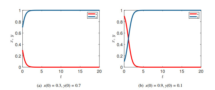
Cooperation is an indispensable behavior in biological systems. In the prisoner's dilemma, due to the individual's selfish psychology, the defector is in the dominant position finally, which results in a social dilemma. In this paper, we discuss the replicator dynamics of the prisoner's dilemma with penalty and mutation. We first discuss the equilibria and stability of the prisoner's dilemma with a penalty. Then, the critical delay of the bifurcation with the payoff delay as the bifurcation parameter is obtained. In addition, considering the case of player mutation based on penalty, we analyze the two-delay system containing payoff delay and mutation delay and find the critical delay of Hopf bifurcation. Theoretical analysis and numerical simulations show that cooperative and defective strategies coexist when only a penalty is added. The larger the penalty is, the more players tend to cooperate, and the critical time delay of the time-delay system decreases with the increase in penalty. The addition of mutation has little effect on the strategy chosen by players. The two-time delay also causes oscillation.

Keywords:

Citation: Yifei Wang, Xinzhu Meng. Evolutionary game dynamics of cooperation in prisoner's dilemma with time delay[J]. Mathematical Biosciences and Engineering, 2023, 20(3): 5024-5042. doi: 10.3934/mbe.2023233

Related Papers:

[1]	José Rodrigo da-Silva, Ana Alexandre, Clarisse Brígido, Solange Oliveira . Can stress response genes be used to improve the symbiotic performance of rhizobia?. AIMS Microbiology, 2017, 3(3): 365-382. doi: 10.3934/microbiol.2017.3.365
[2]	Yen Thi Ngoc Phan, Minh Thuy Tang, Tu Thi Minh Tran, Van Huu Nguyen, Trang Hien Nguyen, Takeshi Tsuruta, Naoki Nishino . Diversity of lactic acid bacteria in vegetable-based and meat-based fermented foods produced in the central region of Vietnam. AIMS Microbiology, 2017, 3(1): 61-70. doi: 10.3934/microbiol.2017.1.61
[3]	Xavier Cruz-González, Nereha Laza-Pérez, Pedro F. Mateos, Raúl Rivas . Analysis and effect of the use of biofertilizers on Trifolium rubens L., a preferential attention species in Castile and Leon, Spain, with the aim of increasing the plants conservation status. AIMS Microbiology, 2017, 3(4): 733-746. doi: 10.3934/microbiol.2017.4.733
[4]	Ángeles Hidalgo, Francisco-Javier López-Baena, José-Enrique Ruiz-Sainz, José-María Vinardell . Studies of rhizobial competitiveness for nodulation in soybean using a non-destructive split-root system. AIMS Microbiology, 2017, 3(2): 323-334. doi: 10.3934/microbiol.2017.2.323
[5]	Jasmine S. Ritschard, Lea Amato, Yadhu Kumar, Britta Müller, Leo Meile, Markus Schuppler . The role of the surface smear microbiome in the development of defective smear on surface-ripened red-smear cheese. AIMS Microbiology, 2018, 4(4): 622-641. doi: 10.3934/microbiol.2018.4.622
[6]	Caroline L. Marden, Ryan McDonald, Harold J. Schreier, Joy E.M. Watts . Investigation into the fungal diversity within different regions of the gastrointestinal tract of Panaque nigrolineatus, a wood-eating fish. AIMS Microbiology, 2017, 3(4): 749-761. doi: 10.3934/microbiol.2017.4.749
[7]	Neda Askari, Hassan Momtaz, Elahe Tajbakhsh . Acinetobacter baumannii in sheep, goat, and camel raw meat: virulence and antibiotic resistance pattern. AIMS Microbiology, 2019, 5(3): 272-284. doi: 10.3934/microbiol.2019.3.272
[8]	Nikolina-Alexandra Xaxiri, Eleni Nikouli, Panagiotis Berillis, Konstantinos Ar. Kormas . Bacterial biofilm development during experimental degradation of Melicertus kerathurus exoskeleton in seawater. AIMS Microbiology, 2018, 4(3): 397-412. doi: 10.3934/microbiol.2018.3.397
[9]	Angel Valverde, María González-Tirante, Marisol Medina-Sierra, Raúl Rivas, Ignacio Santa-Regina, José M. Igual . Culturable bacterial diversity from the chestnut (Castanea sativa Mill.) phyllosphere and antagonism against the fungi causing the chestnut blight and ink diseases. AIMS Microbiology, 2017, 3(2): 293-314. doi: 10.3934/microbiol.2017.2.293
[10]	Mojtaba Moosavian, Mina Moradzadeh, Ataollah Ghadiri, Morteza Saki . Isolation and Identification of Legionella spp. in environmental water sources based on macrophage infectivity potentiator (mip) gene sequencing in southwest Iran. AIMS Microbiology, 2019, 5(3): 223-231. doi: 10.3934/microbiol.2019.3.223

Abstract

1. Introduction

COVID-19 is the novel coronavirus that has spread among humans, mainly in China, since December 2019 ^[1]. It was first discovered in Wuhan, the capital city of the Hubei province ^[2]. The virus subsequently spread to other provinces in China. Cases of infection have also appeared in other countries ^[3,4]. COVID-19 is a respiratory virus that is transferred via contact with an infected person through droplets when a person coughs or sneezes, or through saliva droplets. The main clinical manifestations of the infection are fever, fatigue, respiratory symptoms (mainly dry cough), and emergence of dyspnea. Most patients have mild to moderate symptoms with good prognosis, but some patients can be in critical condition or die ^[1]. As of February 15, 2020, it has been reported that 68,500 people have confirmed with the COVID-19 infection and 1596 people have died in the mainland of China ^[5].

To avoid the risk of a large-scale movement of population that can accelerate the spread of the disease, the Chinese government has implemented various measures. The government keeps track of people who had direct contact with the COVID-19 patients, known as contact tracing. From the last day of contact with a confirmed patient, contacts are monitored for signs of illness within 14 days. If contacts develop fever or other symptoms, they are isolated, tested, and hospitalized immediately to prevent further spread of the virus to others. Since Jan 23, 2020, metropolitan-wide quarantine and traffic restriction have been taken in Wuhan and several nearby cities. As the outbreak grows rapidly, China is imposing a more massive quarantine. All schools have postponed the start of the spring semester. Most companies have also postponed the starting date of work after the holiday of Spring Festival. A number of countries or regions have issued restrictions on the entry of Chinese citizens. A large number of domestic and international flights have been canceled. There is no doubt that the outbreak of this virus infection has severely affected people's life, economy and health. How long this situation will last and when the disease will be controlled is a great concern to everyone.

In the last few decades, there were several major outbreaks of infectious diseases, such as atypical pneumonia (SARS) in 2003, H1N1 influenza in 2009, and H7N9 influenza in 2013. It is imperative to improve early predictive and warning capabilities for the disease endemic or pandemic. Mathematical models, combined with the prevalence data, have been used to study the dynamics, analyze the causes and key factors of the outbreaks, forecast the trend of disease spread, and provide optimal control strategies and measures. For example, Zhou and Ma ^[6] formulated a discrete mathematical model to investigate the transmission of SARS. Their simulation results agree with the data and indicate that early quarantine and a high quarantine rate are crucial to the control of SARS. Chowell et al. ^[7] and Lekone et al. ^[8] developed ordinary differential equations and stochastic SEIR models to study the dynamics of infectious disease and the effect of control interventions, respectively. Their models used the outbreak of Ebola in the Democratic Republic of Congo in 1995 as a case study. Very recently, some researchers have studied the spread of COVID-19 ^[9,10,11]. Most of them estimated the basic reproductive number $R_0$ , a key parameter to evaluate the potential of viral transmission ^{[12,13,14,15,16]}. Tang et al. ^[17,18] constructed a deterministic compartmental model and also estimated the basic reproductive number. They provided the predicted results under different degrees of control measures.

In this study, we will use a discrete-time stochastic compartment model to study the dynamics of COVID-19 epidemics. The model includes the transmission of COVID-19 and the government's measures to control the disease spread. The model captures the epidemiological status of individuals in the clinical progression of the disease and the changes in each time interval. We make full use of the existing reported data and perform parameter estimation based on the data. Furthermore, we forecast the spread of the disease in the next period of time based on the parameter estimates and numerical simulation. We also use simulations to evaluate the risk of returning to work at different timing and provide suggestions on when people can start their routine work and life.

2. Model

Based on the development and epidemiological characteristics of COVID-19 infection, the SEIR model is appropriate to study the dynamic of this disease. The population is partitioned into subpopulations as susceptible ( $S(t)$ ), exposed ( $E(t)$ ), infected ( $I(t)$ ), hospitalized ( $H(t)$ ), and recovered ( $R(t)$ ). Let $N$ denote the total population size. The government takes measures to track and quarantine people who have close contact with confirmed cases. Thus, a fraction of the susceptible population is quarantined and identified as $S_q(t)$ and a fraction of the exposed population is isolated and identified as $E_q(t)$ . We consider the discrete time point series $T = {0, 1, 2, \cdots, T_n}$ as the time progression of the disease. Here the time step is chosen to be one day, $i.e., \ h = 1$ . At this timescale, the number of each compartment is dependent on the number in the previous day and the inflows and removals from other compartments during the day. Let $B_{ij}(t)$ be the number of individual transportation between compartments. We provide their detailed descriptions as follows:

● $B_{11}(t)$ is the number of susceptible individuals who become newly infected;

● $B_{12}(t)$ is the number of quarantined susceptible individuals who have contact with infected individuals but are not infected;

● $B_{21}(t)$ is the number of new cases with symptom onset;

● $B_{31}(t)$ is the number of new confirmed and admitted patients;

● $B_{32}(t)$ is the number of new death from infected individuals;

● $B_{33}(t)$ is the number of newly recovered from infected individuals;

● $B_{41}(t)$ is the number of people released from quarantine;

● $B_{51}(t)$ is the number of people admitted to hospital (also isolated);

● $B_{61}(t)$ is the number of newly recovered from hospitalized cases;

● $B_{62}(t)$ is the number of new death from hospitalized cases.

The transition of an individual from one state to the next state can be considered as a stochastic process. The time length that an individual has been in a certain compartment obeys exponential distribution. If we assume that the parameter of the exponential distribution is $\lambda(t)$ , then the probability that individuals leave the current state in the time interval $h$ is $1-exp(-\lambda (t)h)$ . Further, the numbers of inflows and removals from other compartments during one day can be generated by a binomial distribution. The number of experiments in the binomial distribution is the number of individuals in the current compartment. The transmission of the disease is presumed to occur in the context of close contact between susceptible and infected persons. Assuming the transmission probability is $\beta$ and the contact rate is $c(t)$ , then $\beta c(t)\frac{I(t)}{N}$ is the exponential rate that leads to the probability of individuals leaving the susceptible compartment. In view of contact tracing, we denote the quarantined proportion of individuals exposed to the virus is $q$ . Based on the above assumptions and the stochastic SEIR model in ^[8], the discrete-time stochastic compartment model for COVID-19 infection is constructed as

$\begin{equation} \begin{array}{l} S(t+h) = S(t)-B_{11}(t)-B_{12}(t)+B_{41}(t), \\ E(t+h) = E(t)+(1-q)B_{11}(t)-B_{21}(t), \\ I(t+h) = I(t)+B_{21}(t)-B_{31}(t)-B_{32}(t)-B_{33}(t), \\ S_q(t+h) = S_q(t)+B_{12}(t)-B_{41}(t), \\ E_q(t+h) = E_q(t)+qB_{11}(t)-B_{51}(t), \\ H(t+h) = H(t)+B_{31}(t)+B_{51}(t)-B_{61}(t)-B_{62}(t), \\ R(t+h) = R(t)+B_{33}(t)+B_{61}(t), \\ \end{array} \end{equation}$

(2.1)

where

$\begin{equation*} \begin{array}{l} B_{11}(t)\thicksim Poi(S(t)*P_{11}(t)), \ \ B_{12}(t)\thicksim Poi(S(t)*P_{12}(t)), \\ B_{21}(t)\thicksim Bin(E(t), P_{21}), \ \ B_{31}(t)\thicksim Bin(I(t), P_{31}), \\ B_{32}(t)\thicksim Bin(I(t), P_{32}), \ \ B_{33}(t)\thicksim Bin(I(t), P_{33}), \\ B_{41}(t)\thicksim Bin(S_q(t), P_{41}), \ \ B_{51}(t)\thicksim Bin(E_q(t), P_{51}), \\ B_{61}(t)\thicksim Bin(H(t), P_{61}), \ \ B_{62}(t)\thicksim Bin(H(t), P_{32}).\\ \end{array} \end{equation*}$

The above random variables involve binomial distributions $Bin(n, p)$ with the following probabilities:

$\begin{equation*} \begin{array}{l} P_{11}(t)) = 1-exp[-\beta c(t)\frac{I(t)}{N}h], \ \ P_{12}(t) = 1-exp[-c(t)q(1-\beta)\frac{I(t)}{N}h], \\ P_{21} = 1-exp(-\sigma h), \ \ P_{31} = 1-exp(-\delta_I h), \\ P_{32} = 1-exp(-\alpha h), \ \ P_{33} = 1-exp(-\gamma_I h), \\ P_{41} = 1-exp(-\lambda h), \ \ P_{51} = 1-exp(-\delta_q h), P_{61} = 1-exp(-\gamma_H h).\\ \end{array} \end{equation*}$

Note that the number of $S(t)$ is approximately the total population $N$ in China, which is a large number. The limit distribution of the binomial distribution is the poisson distribution. This is used instead for $B_{11}(t)$ and $B_{12}(t).$ The variation of these seven compartments and their relationship are illustrated in the diagram 1. The other parameters are summarized in Table 1.

Table 1. Estimates of the parameters and initial values of the model.

Parameters	Definition	Baseline values	Range	Mean value	(estimated)Std	Source
$c_0$	Initial contact rate	31	(0, 50]	34.037	0.389	MCMC
$c_u$	Finial contact rate	1	(0, 50]	0.933	0.0037	MCMC
	under control measures
$k$	Exponential decreasing rate	0.1	[0, 1]	0.144	0.0035	MCMC
	of the contact rate
$\beta$	Probability of transmission	0.095	[0, 1]	0.111	0.0015	MCMC
$q$	Quarantine rate of exposed individuals	0.4	[0, 1]	0.415	0.016	MCMC
$\sigma$	Transition rate of exposed individuals	1/7	[0, 1]	1/7	-	^[17]
	to the infected class
$\lambda$	Rate at which the quarantined uninfected	1/14	1/14	1/14	-	^[17]
	contacts were released
$\delta_I$	Transition rate of symptomatic infected	0.1	[0.1]	0.304	0.001	MCMC
	individuals to the quarantined infected class
$\delta_q$	Transition rate of quarantined exposed	0.42	[0, 1]	0.413	0.0116	MCMC
	individuals to the quarantined infected class
$\gamma_I$	Recovery rate of symptomatic infected	0.008	[0, 1]	0.0085	0.0001	MCMC
	individuals
$\gamma_H$	Recovery rate of quarantined infected	0.017	[0, 1]	0.018	0.0003	MCMC
	individuals
$\alpha$	Disease-induced death rate	0.0027	[0, 1]	0.0027	$0.0001$	MCMC
$N$	The total population number	-	-	$1.4\times 10^{10}$	-	$Data$
$E(0)$	Initial exposed population	105	[1,200]	52	0.64	MCMC
$I(0)$	Initial symptomatic infected population	54	[1,100]	31	0.346	MCMC
$S_q(0)$	Initial quarantined susceptible population	-	-	734	-	$Data$
$E_q(0)$	Initial quarantined exposed population	2	[1,100]	5	0.24	MCMC
$H(0)$	Initial quarantined infected population	-	-	41	-	Data
$R(0)$	Initial recovered population	-	-	6	-	Data

| Show Table

DownLoad: CSV

Reducing exposure is one of the effective measures to control the spread of disease. The public raises awareness of precaution and takes fewer trips or wears a mask in the presence of a disease outbreak. The government has taken more control measures, e.g., blocking the entrances and exits of the city to stop the movement of population. In this model, the contact rate $c(t)$ (i.e. the average number of contacts of a person per unit time) is assumed to be a piecewise function. It is a constant before the time point $t^*$ at which control measures are taken. It is assumed to decrease gradually from $c_0$ to $c_u$ . We assume that $c(t)$ takes the following form:

$\begin{equation} c(t) = \left\{\begin{array}{l} c_0, \ \ t\leq t^*, \\ (c_0-c_u)e^{-k(t-t^*)}+c_u, \ \ t > t^*.\\ \end{array}\right. \end{equation}$

(2.2)

The city of Wuhan was blockaded on January 23, 2020. The actual data we used for data fitting start from January 11, 2020. Thus, we let $t^* = 12$ .

3. Data

We obtained the data from the National Health Commission of the People's Republic of China ^[5] and the Health Commission of the Hubei Province ^[19]. The data that will be used for parameter estimation include the cases in the mainland of China, such as the newly reported confirmed cases, the newly recovered cases, the new death cases, and the number of people released from medical observation. The total population $N$ in this study is the population of China, approximately 1.4 billion. The cumulative number of reported confirmed cases can be used to compare with the model simulations. The total number of confirmed cases is the cumulative number of cases minus the cumulative number of recovered and death cases. As a complete reporting coverage of the cases has been available since January 11, 2020, the data used in our analysis are from January 11 to February 13, 2020. Since February 13, the Hubei province has carried out screening of the previous suspected cases and revised the diagnosis results, adding "clinical diagnosis" to the diagnosis classification. Although the number of clinical cases has been public as confirmed cases in Hubei, the clinical diagnosis is not included in the number of confirmed cases in this study.

4. Parameter estimation

In general, Bayesian estimation or the maximum likelihood estimation method can be used to estimate unknown parameters in this type of stochastic models ^[8,20]. Because $B_{ij}(t)$ , where $(i, j)\in$ $\{$ (1, 1), (1, 2), (2, 1), (3, 1), (3, 2), (3, 3), (4, 1), (5, 1), (6, 1), (6, 2) $\}$ , are conditionally independent, the likelihood function can be the accumulation of probability densities of all variables, given by

$\begin{equation} L(B_{11}(t), B_{12}(t), B_{21}(t), B_{31}(t), B_{32}(t), B_{33}(t), B_{41}(t), B_{51}(t), B_{61}(t), B_{62}(t)|\Theta) = \prod\limits_{t = 0}^{T^n}g_{i, j}(B_{ij}(t)|\cdot) \end{equation}$

(4.1)

where $g_{i, j}$ is the binomial densities of $B_{ij}(t)$ . The best scenario is that the value of transportation between compartments can be obtained. However, the exposed and some infected people are impossible to be identified. In the reported cases about COVID-19 infection, the data we obtained is the time series for ${B_{41}, B_{61}, B_{62}}$ , and the number of new cases, which is equal to the sum of $B_{51}$ and $B_{31}$ . The remaining time series including ${B_{11}, B_{12}, B_{21}, B_{32}, B_{33}}$ are hard to be determined. It is difficult to accomplish parameter estimates using Bayesian estimation or the maximum likelihood estimation due to such a data structure. Therefore, the Metropolis-Hastings (MH) algorithm will be used to estimate parameters in our model by carrying out the Markov Chain Monte Carlo (MCMC) procedure ^[21,22].

In the model, we assume $\sigma = 1/7$ and $\lambda = 1/14$ because the quarantined individuals were isolated for 14 days and the incubation period of COVID-19 is about 7 days ^[17,23]. The initial conditions are the data on January 11, that is, $H_0 = 41,$ $R_0 = 6$ , and the sum of $S_q$ and $E_q$ is 739. We estimated the parameters from the mean values of 10,000 samples after a burn-in period of 5000 iterations. The estimated results of all parameters relevant to COVID-19 infection are displayed in Table 1. The model parameters fitted to the data of COVID-19 infection, including the newly reported confirmed cases and the total confirmed cases, are shown in Figure 2. In addition, stochastic simulations in Figure 3 show that the model can provide a good fit to the data of newly recovered cases and new death cases of the COVID-19 infection.

Figure 1. Flow diagram of the COVID-19 infection.

DownLoad: Full-Size Img PowerPoint

Figure 2. The data of newly reported confirmed cases and total number of confirmed cases of COVID-19 disease from January 11, 2020 to February 13, 2020. Stochastic fit was performed 100 times. The newly reported confirmed case data are shown in (a) and the total number of confirmed case data are shown in (b). The data and the fitted are represented by the deep blue and light blue curves, respectively.

DownLoad: Full-Size Img PowerPoint

Figure 3. The data of newly recovered cases and new death cases of COVID-19 disease from January 11 to February 13, 2020. Stochastic fit was performed 100 times. The newly recovered cases are shown in (a), death cases are shown in (b). The data and the fitted are represented by the deep blue and light blue curves, respectively.

DownLoad: Full-Size Img PowerPoint

5. Prediction and control

5.1. The reproductive number

Comparing with the basic reproductive number, the effective reproductive number can be used to measure the number of secondary cases generated by one primary case in a population in which there is partial immunity or some intervention measures have been implemented ^{[24,25,26,27,28]}. It changes during the progress of the disease outbreak. As the population size is much larger than the resulting size of the outbreak, i.e., $S(t)/N\approx1$ , the effective or control reproductive number of our model is given by the following formula

$R_c(t) = \frac{\beta c(t)(1-q)}{\delta_I+\alpha+\gamma_I}.$

In contrast with the basic reproductive number that usually involves a constant contact rate, we use a time-varying contact rate $c(t)$ in the effective reproductive number ^[17]. Using the parameter values estimated from the data fitting, the effective reproductive number $R_c(t)$ can be computed numerically. The result shown in indicates that $R_c(t)$ is large at the beginning of the disease outbreak. However, as control measures are implemented, the effective reproductive number decreases eventually to less than 1.

Figure 4. The effective reproductive number

$R_c(t)$ from January 11 to February 13, 2020. The gray line is the range due to disturbance in the stochastic model.

DownLoad: Full-Size Img PowerPoint

5.2. Prediction

An assumption of our model is that the contact rate is exponentially decreasing to $c_u$ due to various prevention measures. The estimates show that the maximum value of the contact rate is 34.03 at the beginning of disease spread. As control measures are implemented, the contact rate declines to 0.93. This indicates that susceptible people are well protected by these measures and there is a small chance of transmission by infected people. Using this assumption and estimated parameters, we can make predictions about the future trend of the disease spread. In Figure 5(a) and (b), the simulations show the dynamics of the number of newly confirmed cases and the total confirmed cases in the 350 days after January 11, 2020. The number of newly cases has begun to decrease slightly compared with before. Figure 5(a) also indicates that the number of newly confirmed cases will continue to decline in the future. The number of newly confirmed cases will decrease to 0 in about 102–119 days after January 11, i.e., April 22, 2020 to May 9, 2020. Figure 5(b) shows that the number of total confirmed cases is still increasing. It will reach the peak in about 46–48 days after January 11, that is, February 26, 2020 to February 28, 2020.

Figure 5. Predicted results of newly confirmed cases shown in (a) and total number of confirmed cases shown in (b) under control measures in the 350 days since January 11, 2020. The red dotted line in (a) is the time when the newly confirmed cases reach zero. The red dotted line in (b) is the time when the total confirmed cases reach the peak level.

DownLoad: Full-Size Img PowerPoint

5.3. Control measure

Up to now, the Chinese government has adopted very strict measures to control the spread of the disease. Most people are quarantined at home. Most companies have stopped working and all schools have postponed the opening date. How long will such measures last? If people start to work and students go to school as usual, the population flow will increase the risk of contact. Will this lead to a second outbreak of the disease? When does people's life can go back to normal? These are issues of great concern to everybody in the country. We consider the following four scenarios:

$\bf(i).$ Suppose the time to return to work is March 1 but the protective measures are inadequate. The parameters in the model are assumed to be $c(t) = 3$ when $T > 50$ ;

$\bf(ii).$ Suppose the time to return to work is March 1 and the protective measures are good. The parameters are chosen to be $c(t) = 1.5$ when $T > 50$ ;

$\bf(iii).$ Suppose the time to return to work is March 20 but the protective measures are inadequate. The parameters are $c(t) = 3$ when $T > 70$ ;

$\bf (iv).$ Suppose the time to return to work is March 20 and the protective measures are good. The parameters are $c(t) = 1.5$ when $T > 70$ ;

Using the above assumptions and fixing other parameters according to data fitting, we numerically investigate the dynamics of the number of newly confirmed cases and total confirmed cases, which are shown in Figure 6. The simulations suggest that when people return to work early without sufficient protection it is likely to observe the increase of newly confirmed cases. The total number of confirmed cases will also increase by more than 2000. If people return to work on March 20, it will result in a small increase in the number of newly confirmed cases. However, it's going to decrease quickly. Thus, postponing the return to work would be of great help to control the disease transmission.

Figure 6. Predicted results of newly confirmed cases shown in (a) and total number of confirmed cases shown in (b) with four assumptions (see text) in the 350 days since January 11, 2020. The results are the mean of 50 stochastic simulations.

DownLoad: Full-Size Img PowerPoint

6. Discussion

In view of the randomness in the transmission of the COVID-19 infection, we construct a discrete-time stochastic compartment system to study the dynamic behavior of the disease outbreak, in which the population in each compartment is assumed to obey a binomial distribution. In the model, we further assume that the contact rate between susceptible and infected individuals decreases exponentially since the government has implemented strict control measures. This discrete system can make a good use of the newly reported data, including the number of newly reported confirmed cases, newly recovered cases, new death cases, and those quarantined that are released per day, to calibrate the model parameters. Because the diagnostic criterion for confirmed cases was revised on February 13, we use the data reported from January 11 to February 13, 2020 in this study. Although there are no data for the populations in the other groups, we estimated the parameters in the model using the MCMC procedure based on the exiting reported data.

The maximum value of contact rate we estimated is 34.02 and then dropped to 0.93. It indicates that the control measures implemented are very effective. shows that the effective reproductive number of the infection declines from 6.96 to 0.47 over the time period of simulation. Some other groups have also estimated $R_0$ of the COVID-19 infection ^[29,30]. See a summary of the estimates in the reference ^[31]. Some estimates of $R_0$ are comparable to ours (before various control measures are taken) and some are smaller. This may be due to different estimation methods under different model assumptions. In any case, the results indicate that this novel coronavirus is highly contagious in the early stage (e.g., higher than the SARS coronavirus outbreak in 2003 ^[31]). However, the control measures implemented so far are shown to be efficient in lowering the effective reproductive number to below 1.

The stochastic fits show that the reported data are less than those simulated in the initial phase, but the subsequent simulation agrees well with the reported data. Most of the data are in the region of the stochastic simulation. By the time of the submission of this manuscript, the number of newly reported confirmed cases has begun to decrease. Assuming that the current control measures adopted by the government and individuals are maintained, the predicted results shown in Figure 4 indicate that the peak of total confirmed cases will reach around late February of 2020, followed by a decrease. The newly confirmed cases will decline to zero in late April or early May of 2020. To study the timing of returning to work on the disease dynamics, we consider four different scenarios on the time to return to work and the strength of protective measures. We assume the contact rate is 3 if the resumption of work causes wide migration of people and the protective measures are not sufficient. In this case, the simulation shows that the infection will have a second outbreak if people return to work on March 1. The situation will be better if people can return to work after March 20, 2020.

In conclusion, our simulation shows that the contact rate is a key factor on the control of the COVID-19 outbreak. When there is a sign of epidemic, we should raise awareness of self-protection and take all possible protective measures, such as wearing a mask and staying indoor to reduce the risk of getting infected. Although the number of new cases of infection is decreasing, there is still a possibility of future outbreaks if there are no adequate protective measures or people return to work early. The public should not relax their vigilance against the transmission of this highly contagious disease.

Acknowledgment

This research was partially supported by the National Natural Science Foundation of China (grant numbers: 61772017 (ST), 11631012 (ST)) and by the Fundamental Research Funds for the Central Universities (grant numbers: 2018CBLZ001 (SH), GK201901008 (ST)). L. Rong is supported by the National Science Foundation (grant number: DMS-1758290).

Conflict of interest

No conflict of interest.

References

[1]	J. W. Weibull, Evolutionary Game Theory, MIT press, 1997.
[2]	J. M. Smith, Evolution and the Theory of Games, Cambridge university press, 1982.
[3]	J. Tanimoto, Fundamentals of Rvolutionary Game Theory and its Applications, Springer Japan, 2015.
[4]	J. M. Smith, G. R. Price, The logic of animal conflict, Nature, 246 (1973), 15–18. https://doi.org/10.1038/246015a0
[5]	R. Axelrod, W. D. Hamilton, The evolution of cooperation, Science, 211 (1981), 1390–1396. https://www.science.org/doi/abs/10.1126/science.7466396
[6]	W. Zhang, Y. S. Li, C. Xu, P. M. Hui, Cooperative behavior and phase transitions in co-evolving stag hunt game, Phys. A, 443 (2016), 161–169. https://doi.org/10.1016/j.physa.2015.09.047 doi: 10.1016/j.physa.2015.09.047
[7]	J. M. Du, Z. R. Wu, Evolutionary dynamics of cooperation in dynamic networked systems with active striving mechanism, Appl. Math. Comput., 430 (2022), 127295. https://doi.org/10.1016/j.amc.2022.127295 doi: 10.1016/j.amc.2022.127295
[8]	R. Chiong, M. Kirley, Random mobility and the evolution of cooperation in spatial N-player iterated Prisoner's Dilemma games, Phys. A, 391 (2012), 3915–3923. https://doi.org/10.1016/j.physa.2012.03.010 doi: 10.1016/j.physa.2012.03.010
[9]	J. L. Chen, X. W. Liu, H. Z. Wang, J. Yang, The disconnection-reconnection-elite mechanism enhances cooperation of evolutionary game on lattice, Chaos Solitons Fractals, 157 (2022), 111897. https://doi.org/10.1016/j.chaos.2022.111897 doi: 10.1016/j.chaos.2022.111897
[10]	J. X. Pi, G. H. Yang, H. Yang, Evolutionary dynamics of cooperation in N-person snowdrift games with peer punishment and individual disguise, Phys. A, 592 (2022), 126839. https://doi.org/10.1016/j.physa.2021.126839 doi: 10.1016/j.physa.2021.126839
[11]	P. C. Zhu, H. Guo, H. L. Zhang, Y. Han, Z. Wang, C. Chu, The role of punishment in the spatial public goods game, Nonlinear Dyn., 102 (2020), 2959–2968. https://doi.org/10.1007/s11071-020-05965-0 doi: 10.1007/s11071-020-05965-0
[12]	P. Catalán, J. M. Seoane, M. A. Sanjuán, Mutation-selection equilibrium in finite populations playing a Hawk–Dove game, Commun. Nonlinear Sci. Numer. Simul., 25 (2015), 66–73. https://doi.org/10.1016/j.cnsns.2015.01.012 doi: 10.1016/j.cnsns.2015.01.012
[13]	T. Nagatani, G. Ichinose, K. I. Tainaka, Metapopulation model for rock–paper–scissors game: mutation affects paradoxical impacts, J. Theor. Biol., 450 (2018), 22–29. https://doi.org/10.1016/j.jtbi.2018.04.005 doi: 10.1016/j.jtbi.2018.04.005
[14]	T. A. Wettergren, Replicator dynamics of an N-player snowdrift game with delayed payoffs, Appl. Math. Comput., 404 (2021), 126204. https://doi.org/10.1016/j.amc.2021.126204 doi: 10.1016/j.amc.2021.126204
[15]	J. Alboszta, J. Miekisz, Stability of evolutionarily stable strategies in discrete replicator dynamics with time delay, J. Theor. Biol., 231 (2004), 175–179. https://doi.org/10.1016/j.jtbi.2004.06.012 doi: 10.1016/j.jtbi.2004.06.012
[16]	J. Miekisz, S. Wesołowski, Stochasticity and time delays in evolutionary games, Dyn. Games Appl., 1 (2011), 440–448. https://doi.org/10.1007/s13235-011-0028-1 doi: 10.1007/s13235-011-0028-1
[17]	J. Burridge, Y. Gao, Y. Mao, Delayed response in the Hawk Dove game, Eur. Phys. J. B, 90 (2017), 1–6. https://doi.org/10.1140/epjb/e2016-70471-1 doi: 10.1140/epjb/e2016-70471-1
[18]	S. Mittal, A. Mukhopadhyay, S. Chakraborty, Evolutionary dynamics of the delayed replicator-mutator equation: Limit cycle and cooperation, Phys. Rev. E, 101 (2020), 042410. https://doi.org/10.1103/PhysRevE.101.042410 doi: 10.1103/PhysRevE.101.042410
[19]	L. M. Hu, X. L. Qiu, Stability analysis of game models with fixed and stochastic delays, Appl. Math. Comput., 435 (2022), 127473. https://doi.org/10.1016/j.amc.2022.127473 doi: 10.1016/j.amc.2022.127473
[20]	J. Tanimoto, H. Sagara, Relationship between dilemma occurrence and the existence of a weakly dominant strategy in a two-player symmetric game, Biosystems, 90 (2007), 105–114. https://doi.org/10.1016/j.biosystems.2006.07.005 doi: 10.1016/j.biosystems.2006.07.005
[21]	Z. Wang, S. Kokubo, M. Jusup, J. Tanimoto, Universal scaling for the dilemma strength in evolutionary games, Phys. Life Rev., 14 (2015), 1–30. https://doi.org/10.1016/j.plrev.2015.04.033 doi: 10.1016/j.plrev.2015.04.033
[22]	H. Ito, J. Tanimoto, Scaling the phase-planes of social dilemma strengths shows game-class changes in the five rules governing the evolution of cooperation, R. Soc. Open Sci., 5 (2018), 181085. https://doi.org/10.1098/rsos.181085 doi: 10.1098/rsos.181085
[23]	M. R. Arefin, K. M. A. Kabir, M. Jusup, et al. Social efficiency deficit deciphers social dilemmas, Sci. Rep., 10 (2020), 16092. https://doi.org/10.1038/s41598-020-72971-y doi: 10.1038/s41598-020-72971-y
[24]	J. Tanimoto, Sociophysics Approach to Epidemics, Singapore, Springer, 2021.
[25]	M. Doebeli, C. Hauert, Models of cooperation based on the Prisoner's Dilemma and the Snowdrift game, Ecol. Lett., 8 (2005), 748–766. https://doi.org/10.1111/j.1461-0248.2005.00773.x doi: 10.1111/j.1461-0248.2005.00773.x
[26]	S. Fan, A new extracting formula and a new distinguishing means on the one variable cubic equation, Nat. Sci. J. Hainan Teach. Coll, 2 (1989), 91–98.
[27]	S. Zhang, R. Clark, Y. K. Huang, Frequency-dependent strategy selection in a hunting game with a finite population, Appl. Math. Comput., 382 (2020), 125355. https://doi.org/10.1016/j.amc.2020.125355 doi: 10.1016/j.amc.2020.125355
[28]	F. Yan, X. Chen, Z. Qiu, A. Szolnoki, Cooperator driven oscillation in a time-delayed feedback-evolving game, New J. Phys., 23 (2021), 053017. https://dx.doi.org/10.1088/1367-2630/abf205 doi: 10.1088/1367-2630/abf205
[29]	D. Pais, C. H. Caicedo-Nunez, N. E. Leonard, Hopf bifurcations and limit cycles in evolutionary network dynamics, SIAM J. Appl. Dyn. Syst., 11 (2012). 1754–1784. https://doi.org/10.1137/120878537
[30]	A. Szolnoki, M. Perc, Decelerated invasion and waning-moon patterns in public goods games with delayed distribution, Phys. Rev. E, 87 (2013), 054801. https://doi.org/10.1103/PhysRevE.87.054801 doi: 10.1103/PhysRevE.87.054801
[31]	X. W. Wang, S. Nie, L. L. Jiang, B. H. Wang, S. M. Chen, Role of delay-based reward in the spatial cooperation, Phys. A, 456 (2017), 153–158. https://doi.org/10.1016/j.physa.2016.08.014 doi: 10.1016/j.physa.2016.08.014
[32]	D. Helbing, A. Szolnoki, M. Perc, G. Szabó, Evolutionary establishment of moral and double moral standards through spatial interactions, PLoS Comput. Biol., 6 (2010), e1000758. https://doi.org/10.1371/journal.pcbi.1000758 doi: 10.1371/journal.pcbi.1000758
[33]	D. Helbing, A. Szolnoki, M. Perc, G. Szabó, Punish, but not too hard: how costly punishment spreads in the spatial public goods game, New J. Phys., 12 (2010), 083005. https://doi.org/10.1088/1367-2630/12/8/083005 doi: 10.1088/1367-2630/12/8/083005
[34]	X. Chen, A. Szolnoki, M. Perc, Probabilistic sharing solves the problem of costly punishment, New J. Phys., 16 (2014), 083016. https://doi.org/10.1088/1367-2630/16/8/083016 doi: 10.1088/1367-2630/16/8/083016
[35]	L. Stella, W. Baar, D. Bauso, Lower network degrees promote cooperation in the prisoner's dilemma with environmental feedback, IEEE Contr. Syst. Lett., 6 (2022). https://doi.org/10.1109/LCSYS.2022.3175402
[36]	L. Stella, D. Bauso, The Impact of irrational behaviours in the optional prisoner's dilemma with game-environment feedback, Int. J. Robust Nonlinear Control, 2022 (2022). https://doi.org/10.1002/rnc.5935
[37]	X. R. Mao, G. Marion, E. Renshaw, Environmental Brownian noise suppresses explosions in population dynamics, Stochastic Processes Appl., 97 (2002), 95–110. https://doi.org/10.1016/S0304-4149(01)00126-0 doi: 10.1016/S0304-4149(01)00126-0

This article has been cited by:

1.	Millicent R. Smith, Idupulapati M. Rao, 2021, 9780128191941, 384, 10.1016/B978-0-12-819194-1.00012-8
2.	A. H. Gunnabo, J. van Heerwaarden, R. Geurts, E. Wolde-meskel, T. Degefu, K. E. Giller, Phylogeography and Symbiotic Effectiveness of Rhizobia Nodulating Chickpea (Cicer arietinum L.) in Ethiopia, 2021, 81, 0095-3628, 703, 10.1007/s00248-020-01620-8
3.	Mark A. Uebersax, Karen A. Cichy, Francisco E. Gomez, Timothy G. Porch, Jim Heitholt, Juan M. Osorno, Kelvin Kamfwa, Sieglinde S. Snapp, Scott Bales, Dry beans ( Phaseolus vulgaris L.) as a vital component of sustainable agriculture and food security—A review , 2022, 2639-6181, 10.1002/leg3.155
4.	Ravinder K. Goyal, Autar K. Mattoo, Maria Augusta Schmidt, Rhizobial–Host Interactions and Symbiotic Nitrogen Fixation in Legume Crops Toward Agriculture Sustainability, 2021, 12, 1664-302X, 10.3389/fmicb.2021.669404
5.	Anna Szczerba, Agnieszka Płażek, Przemysław Kopeć, Magdalena Wójcik-Jagła, Franciszek Dubert, Effect of different Bradyrhizobium japonicum inoculants on physiological and agronomic traits of soybean (Glycine max (L.) Merr.) associated with different expression of nodulation genes, 2024, 24, 1471-2229, 10.1186/s12870-024-05911-x

Reader Comments

Your name:*

Email:*
© 2023 the Author(s), licensee AIMS Press. This is an open access article distributed under the terms of the Creative Commons Attribution License (http://creativecommons.org/licenses/by/4.0)