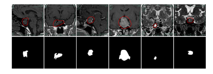
Pituitary adenoma is a common neuroendocrine neoplasm, and most of its MR images are characterized by blurred edges, high noise and similar to surrounding normal tissues. Therefore, it is extremely difficult to accurately locate and outline the lesion of pituitary adenoma. To sovle these limitations, we design a novel deep learning framework for pituitary adenoma MRI image segmentation. Under the framework of U-Net, a newly cross-layer connection is introduced to capture richer multi-scale features and contextual information. At the same time, full-scale skip structure can reasonably utilize the above information obtained by different layers. In addition, an improved inception-dense block is designed to replace the classical convolution layer, which can enlarge the effectiveness of the receiving field and increase the depth of our network. Finally, a novel loss function based on binary cross-entropy and Jaccard losses is utilized to eliminate the problem of small samples and unbalanced data. The sample data were collected from 30 patients in Quzhou People's Hospital, with a total of 500 lesion images. Experimental results show that although the amount of patient sample is small, the proposed method has better performance in pituitary adenoma image compared with existing algorithms, and its Dice, Intersection over Union (IoU), Matthews correlation coefficient (Mcc) and precision reach 88.87, 80.67, 88.91 and 97.63%, respectively.
Citation: Xiaoliang Jiang, Junjian Xiao, Qile Zhang, Lihui Wang, Jinyun Jiang, Kun Lan. Improved U-Net based on cross-layer connection for pituitary adenoma MRI image segmentation[J]. Mathematical Biosciences and Engineering, 2023, 20(1): 34-51. doi: 10.3934/mbe.2023003
Pituitary adenoma is a common neuroendocrine neoplasm, and most of its MR images are characterized by blurred edges, high noise and similar to surrounding normal tissues. Therefore, it is extremely difficult to accurately locate and outline the lesion of pituitary adenoma. To sovle these limitations, we design a novel deep learning framework for pituitary adenoma MRI image segmentation. Under the framework of U-Net, a newly cross-layer connection is introduced to capture richer multi-scale features and contextual information. At the same time, full-scale skip structure can reasonably utilize the above information obtained by different layers. In addition, an improved inception-dense block is designed to replace the classical convolution layer, which can enlarge the effectiveness of the receiving field and increase the depth of our network. Finally, a novel loss function based on binary cross-entropy and Jaccard losses is utilized to eliminate the problem of small samples and unbalanced data. The sample data were collected from 30 patients in Quzhou People's Hospital, with a total of 500 lesion images. Experimental results show that although the amount of patient sample is small, the proposed method has better performance in pituitary adenoma image compared with existing algorithms, and its Dice, Intersection over Union (IoU), Matthews correlation coefficient (Mcc) and precision reach 88.87, 80.67, 88.91 and 97.63%, respectively.

| [1] |
J. Feng, H. Gao, Q. Zhang, Y. Zhou, C. Li, S. Zhao, et al., Metabolic profiling reveals distinct metabolic alterations in different subtypes of pituitary adenomas and confers therapeutic targets, J. Transl. Med., 17 (2019), 1–13. https://doi.org/10.1186/s12967-019-2042-9 doi: 10.1186/s12967-019-2042-9

|
| [2] |
X. M. Liu, Q. Yuan, Y. Z Gao, K. L. He, S. Wang, X. Tang, et al., Weakly supervised segmentation of COVID-19 infection with scribble annotation on CT images, Pattern Recognit., 122 (2022), 108341. https://doi.org/10.1016/j.patcog.2021.108341 doi: 10.1016/j.patcog.2021.108341
|
| [3] |
B. J. Kar, M. V. Cohen, S. P. McQuiston, C. M. Malozzi, A deep-learning semantic segmentation approach to fully automated MRI-based left-ventricular deformation analysis in cardiotoxicity, Magn. Reson. Imaging, 78 (2021), 127–139. https://doi.org/10.1016/j.mri.2021.01.005 doi: 10.1016/j.mri.2021.01.005
|
| [4] |
N. Mu, H. Y. Wang, Y. Zhang, J. F. Jiang, J. S. Tang, Progressive global perception and local polishing network for lung infection segmentation of COVID-19 CT images, Pattern Recognit., 120 (2021), 108168. https://doi.org/10.1016/j.patcog.2021.108168 doi: 10.1016/j.patcog.2021.108168
|
| [5] |
X. M. Liu, Z. S. Guo, J. Cao, J. S. Tang, MDC-net: A new convolutional neural network for nucleus segmentation in histopathology images with distance maps and contour information, Comput. Biol. Med., 135 (2021), 104543. https://doi.org/10.1016/j.compbiomed.2021.104543 doi: 10.1016/j.compbiomed.2021.104543
|
| [6] |
H. M. Rai, K. Chatterjee, S. Dashkevich, Automatic and accurate abnormality detection from brain MR images using a novel hybrid UnetResNext-50 deep CNN model, Biomed. Signal Process. Control, 66 (2021), 102477. https://doi.org/10.1016/j.bspc.2021.102477 doi: 10.1016/j.bspc.2021.102477
|
| [7] | O. Ronneberger, P. Fischer, T. Brox, U-Net: Convolutional networks for biomedical image segmentation, in International Conference on Medical Image Computing and Computer-assisted Intervention, Springer, Cham, (2015), 234–241. https://doi.org/10.1007/978-3-319-24574-4_28 |
| [8] | S. Xie, R. Girshick, P. Dollár, Z. Tu, K. He, Aggregated residual transformations for deep neural networks, in IEEE Conference on Computer Vision and Pattern Recognition, Honolulu, HI, USA, (2017), 5987–5995. https://doi.org/10.1016/j.cmpb.2021.106566 |
| [9] |
H. C. Lu, S. W. Tian, L. Yu, L. Liu, J. L. Cheng, W. D. Wu, et al., DCACNet: Dual context aggregation and attention-guided cross deconvolution network for medical image segmentation, Comput. Methods Programs Biomed., 214 (2022), 106566. https://doi.org/10.1016/j.cmpb.2021.106566 doi: 10.1016/j.cmpb.2021.106566
|
| [10] |
M. U. Rehman, S. Cho, J. Kim, K. T. Chong, BrainSeg-Net: Brain tumor MR image segmentation via enhanced encoder-decoder network, Diagnostics, 11 (2021), 169. https://doi.org/10.3390/diagnostics11020169 doi: 10.3390/diagnostics11020169
|
| [11] |
P. Tang, C. Zu, M. Hong, R. Yan, X. C. Peng, J. H. Xiao, et al., DA-DSUnet: Dual attention-based dense SU-Net for automatic head-and-neck tumor segmentation in MRI images, Neurocomputing, 435 (2021), 103–113. https://doi.org/10.1016/j.neucom.2020.12.085 doi: 10.1016/j.neucom.2020.12.085
|
| [12] |
U. Latif, A. R. Shahid, B. Raza, S. Ziauddin, M. A. Khan, An end-to-end brain tumor segmentation system using multi-inception-UNet, Int. J. Imaging Syst. Technol., 31 (2021), 1803–1816. https://doi.org/10.1002/ima.22585 doi: 10.1002/ima.22585
|
| [13] |
X. F. Du, J. S. Wang, W. Z. Sun, Densely connected U-Net retinal vessel segmentation algorithm based on multi-scale feature convolution extraction, Med. Phys., 48 (2021), 3827–3841. https://doi.org/10.1002/mp.14944 doi: 10.1002/mp.14944
|
| [14] |
Z. Y. Wang, Y. J. Peng, D. P. Li, Y. F. Guo, B. Zhang, MMNet: A multi-scale deep learning network for the left ventricular segmentation of cardiac MRI images, Appl. Intell., 52 (2022), 5225–5240. https://doi.org/10.1007/s10489-021-02720-9 doi: 10.1007/s10489-021-02720-9
|
| [15] |
M. Yang, H. W. Wang, K. Hu, G. Yin, Z. Q. Wei, IA-Net: An inception-attention-module-based network for classifying underwater images from others, IEEE J. Oceanic Eng., 47 (2022), 704–717. https://doi.org/10.1109/JOE.2021.3126090 doi: 10.1109/JOE.2021.3126090
|
| [16] |
J. S. Zhou, Y. W. Lu, S. Y. Tao, X. Cheng, C. X. Huang, E-Res U-Net: An improved U-Net model for segmentation of muscle images, Expert Syst. Appl., 185 (2021), 115625. https://doi.org/10.1016/j.eswa.2021.115625 doi: 10.1016/j.eswa.2021.115625
|
| [17] |
S. Y. Chen, Y. N. Zou, P. X. Liu, IBA-U-Net: Attentive BConvLSTM U-Net with redesigned inception for medical image segmentation, Comput. Biol. Med., 135 (2021), 104551. https://doi.org/10.1016/j.compbiomed.2021.104551 doi: 10.1016/j.compbiomed.2021.104551
|
| [18] |
F. Hoorali, H. Khosravi, B. Moradi, IRUNet for medical image segmentation, Expert Syst. Appl., 191 (2022), 116399. https://doi.org/10.1016/j.eswa.2021.116399 doi: 10.1016/j.eswa.2021.116399
|
| [19] |
Z. Zhang, C. D. Wu, S. Coleman, D. Kerr, Dense-inception U-Net for medical image segmentation, Comput. Biol. Med., 192 (2020), 105395. https://doi.org/10.1016/j.cmpb.2020.105395 doi: 10.1016/j.cmpb.2020.105395
|
| [20] |
S. A. Bala, S. Kant, Dense dilated inception network for medical image segmentation, Int. J. Adv. Comput. Sci. Appl., 11 (2020), 785–793. https://doi.org/10.14569/IJACSA.2020.0111195 doi: 10.14569/IJACSA.2020.0111195
|
| [21] |
L. Wang, J. Gu, Y. Chen, Y. Liang, W. Zhang, J. Pu, et al., Automated segmentation of the optic disc from fundus images using an asymmetric deep learning network, Pattern Recognit., 112 (2021), 107810. https://doi.org/10.1016/j.patcog.2020.107810 doi: 10.1016/j.patcog.2020.107810
|
| [22] |
Z. Zheng, Y. Wan, Y. Zhang, S. Xiang, D. Peng, B. Zhang, CLNet: Cross-layer convolutional neural network for change detection in optical remote sensing imagery, ISPRS J. Photogramm. Remote Sens., 175 (2021), 247–267. https://doi.org/10.1016/j.isprsjprs.2021.03.005 doi: 10.1016/j.isprsjprs.2021.03.005
|
| [23] | H. S. Zhao, J. P. Shi, X. J. Qi, X. G. Wang, J. Y. Jia, Pyramid scene parsing network, in IEEE Conference on Computer Vision and Pattern Recognition, (2017), 6230–6239. |
| [24] |
S. Ran, J. Ding, B. Liu, X. Ge, G. Ma, Multi-U-Net: Residual module under multisensory field and attention mechanism based optimized U-Net for VHR image semantic segmentation, Sensors, 21 (2021), 1794. https://doi.org/10.3390/s21051794 doi: 10.3390/s21051794
|
| [25] |
R. M. Rad, P. Saeedi, J. Au, J. Havelock, Trophectoderm segmentation in human embryo images via inceptioned U-Net, Med. Image Anal., 62 (2020), 101612. https://doi.org/10.1016/j.media.2019.101612 doi: 10.1016/j.media.2019.101612
|
| [26] |
N. S. Punn, S. Agarwal, Multi-modality encoded fusion with 3d inception u-net and decoder model for brain tumor segmentation, Multimed. Tools Appl., 80 (2020), 30305–30320. https://doi.org/10.1007/s11042-020-09271-0 doi: 10.1007/s11042-020-09271-0
|
| [27] | Z. W. Zhou, M. M. R. Siddiquee, N. Tajbakhsh. J. M. Liang, UNet++: A nested U-Net architecture for medical image segmentation, in Deep Learning in Medical Image Analysis and Multimodal Learning for Clinical Decision Support, (2018), 3–11. https://doi.org/10.1007/978-3-030-00889-5_1 |
| [28] |
B. Zuo, F. F. Lee, Q. Chen, An efficient U-shaped network combined with edge attention module and context pyramid fusion for skin lesion segmentation, Med. Biol. Eng. Comput., 60 (2022), 1987–2000. https://doi.org/10.1007/s11517-022-02581-5 doi: 10.1007/s11517-022-02581-5
|
| [29] |
D. P. Li, Y. J. Peng, Y. F. Guo, J. D. Sun, MFAUNet: Multiscale feature attentive U-Net for cardiac MRI structural segmentation, IET Image Proc., 16 (2022), 1227–1242. https://doi.org/10.1049/ipr2.12406 doi: 10.1049/ipr2.12406
|
| [30] |
V. S. Bochkov, L. Y. Kataeva, wUUNet: Advanced fully convolutional neural network for multiclass fire segmentation, Symmetry, 13 (2021), 98. https://doi.org/10.3390/sym13010098 doi: 10.3390/sym13010098
|
| [31] |
D. John, C. Zhang, An attention-based U-Net for detecting deforestation within satellite sensor imagery, Int. J. Appl. Earth Obs. Geoinf., 107 (2022), 102685. https://doi.org/10.1016/j.jag.2022.102685 doi: 10.1016/j.jag.2022.102685
|
| [32] |
Y. Y. Yang, C. Feng, R. F. Wang, Automatic segmentation model combining U-Net and level set method for medical images, Expert Syst. Appl., 153 (2020), 113419. https://doi.org/10.1016/j.eswa.2020.113419 doi: 10.1016/j.eswa.2020.113419
|
| [33] |
I. Ahmed, M. Ahmad, G. Jeon, A real-time efficient object segmentation system based on u-net using aerial drone images, J. Real-Time Image Process., 18 (2021), 1745–1758. https://doi.org/10.1007/s11554-021-01166-z doi: 10.1007/s11554-021-01166-z
|
| [34] |
M. Jiang, F. Zhai, J. Kong, A novel deep learning model DDU-net using edge features to enhance brain tumor segmentation on MR images, Artif. Intell. Med., 121 (2021), 102180. https://doi.org/10.1016/j.artmed.2021.102180 doi: 10.1016/j.artmed.2021.102180
|
| [35] |
D. Li, A. Cong, S. Guo, Sewer damage detection from imbalanced CCTV inspection data using deep convolutional neural networks with hierarchical classification, Autom. Constr., 101 (2019), 199–208. https://doi.org/10.1016/j.autcon.2019.01.017 doi: 10.1016/j.autcon.2019.01.017
|
| [36] |
M. M. Ji, Z. B. Wu, Automatic detection and severity analysis of grape black measles disease based on deep learning and fuzzy logic, Comput. Electron. Agric., 193 (2022), 106718. https://doi.org/10.1016/j.compag.2022.106718 doi: 10.1016/j.compag.2022.106718
|
| [37] | O. Oktay, J. Schlemper, L. L. Folgoc, M. Lee, M. Heinrich, K. Misawa, et al., Attention U-Net: Learning where to look for the pancreas, preprint, arXiv: 1804.03999. |
| [38] | G. Huang, Z. Liu, V. Laurens, K. Q. Weinberger, Densely connected convolutional networks, in IEEE Conference on Computer Vision and Pattern Recognition, (2017), 2261–2269. https://doi.org/10.1109/CVPR.2017.243 |
| [39] | A. Paszke, A. Chaurasia, S. Kim, E. Culurciello, ENet: A deep neural network architecture for real-time semantic segmentation, preprint, arXiv: 1606.02147. |
| [40] | K. Sun, B. Xiao, D. Liu, J. D. Wang, Deep high-resolution representation learning for human pose estimation, in Proceedings of the IEEE/CVF Conference on Computer Vision and Pattern Recognition, (2019), 5693–5703. https://doi.org/10.1109/CVPR.2019.00584 |
| [41] | H. H. Zhao, X. J. Qi, X. Y. Shen, J. P. Shi, J. Y. Jia, ICNet for real-time semantic segmentation on high-resolution images, in Proceedings of the European Conference on Computer Vision, (2018), 405–420. |
| [42] | M. Z. Alom, M. Hasan, C. Yakopcic, T. M. Taha, V. K. Asari, Recurrent residual convolutional neural network based on U-Net (R2U-Net) for medical image segmentation, preprint, arXiv: 1802.06955. |
| [43] |
V. Badrinarayanan, A. Kendall, R. Cipolla, SegNet: A deep convolutional encoder-decoder architecture for image segmentation, IEEE Trans. Pattern Anal. Mach. Intell., 39 (2017), 2481–2495. https://doi.org/10.1109/TPAMI.2016.2644615 doi: 10.1109/TPAMI.2016.2644615
|
| [44] | J. Bullock, C. Cuesta-Lázaro, A. Quera-Bofarull, XNet: A convolutional neural network (CNN) implementation for medical X-Ray image segmentation suitable for small datasets, in Medical Imaging 2019: Biomedical Applications in Molecular, Structural, and Functional Imaging, (2019), 453–463. https://doi.org/10.1117/12.2512451 |
| [45] | H. Huang, L. Lin, R. Tong, H. Hu, J. Wu, UNet 3+: A full-scale connected UNet for medical image segmentation, in IEEE International Conference on Acoustics, Speech and Signal Processing, (2020), 1055–1059. https://doi.org/10.1109/ICASSP40776.2020.9053405 |
| [46] |
P. Tschandl, C. Rosendahl, H. Kittler, The HAM10000 dataset, a large collection of multi-source dermatoscopic images of common pigmented skin lesions, Sci. Data, 5 (2018), 180161. https://doi.org/10.1038/sdata.2018.161 doi: 10.1038/sdata.2018.161
|


Figures(10) / Tables(7)

Xiaoliang Jiang, Junjian Xiao, Qile Zhang, Lihui Wang, Jinyun Jiang, Kun Lan. Improved U-Net based on cross-layer connection for pituitary adenoma MRI image segmentation[J]. Mathematical Biosciences and Engineering, 2023, 20(1): 34-51. doi: 10.3934/mbe.2023003


 DownLoad: