Calcified aortic valve stenosis (CAVS) is caused by calcium buildup and tissue thickening that impede the blood flow from left ventricle (LV) to aorta. In recent years, CAVS has become one of the most common cardiovascular diseases. Therefore, it is necessary to study the mechanics of aortic valve (AV) caused by calcification. In this paper, based on a previous idealized AV model, the hybrid immersed boundary/finite element method (IB/FE) is used to study AV dynamics and hemodynamic performance under normal and calcified conditions. The computational CAVS model is realized by dividing the AV leaflets into a calcified region and a healthy region, and each is described by a specific constitutive equation. Our results show that calcification can significantly affect AV dynamics. For example, the elasticity and mobility of the leaflets decrease due to calcification, leading to a smaller opening area with a high forward jet flow across the valve. The calcified valve also experiences an increase in local stress and strain. The increased loading due to AV stenosis further leads to a significant increase in left ventricular energy loss and transvalvular pressure gradients. The model predicted hemodynamic parameters are in general consistent with the risk classification of AV stenosis in the clinic. Therefore, mathematical models of AV with calcification have the potential to deepen our understanding of AV stenosis-induced ventricular dysfunction and facilitate the development of computational engineering-assisted medical diagnosis in AV related diseases.
Citation: Li Cai, Yu Hao, Pengfei Ma, Guangyu Zhu, Xiaoyu Luo, Hao Gao. Fluid-structure interaction simulation of calcified aortic valve stenosis[J]. Mathematical Biosciences and Engineering, 2022, 19(12): 13172-13192. doi: 10.3934/mbe.2022616
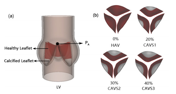
Calcified aortic valve stenosis (CAVS) is caused by calcium buildup and tissue thickening that impede the blood flow from left ventricle (LV) to aorta. In recent years, CAVS has become one of the most common cardiovascular diseases. Therefore, it is necessary to study the mechanics of aortic valve (AV) caused by calcification. In this paper, based on a previous idealized AV model, the hybrid immersed boundary/finite element method (IB/FE) is used to study AV dynamics and hemodynamic performance under normal and calcified conditions. The computational CAVS model is realized by dividing the AV leaflets into a calcified region and a healthy region, and each is described by a specific constitutive equation. Our results show that calcification can significantly affect AV dynamics. For example, the elasticity and mobility of the leaflets decrease due to calcification, leading to a smaller opening area with a high forward jet flow across the valve. The calcified valve also experiences an increase in local stress and strain. The increased loading due to AV stenosis further leads to a significant increase in left ventricular energy loss and transvalvular pressure gradients. The model predicted hemodynamic parameters are in general consistent with the risk classification of AV stenosis in the clinic. Therefore, mathematical models of AV with calcification have the potential to deepen our understanding of AV stenosis-induced ventricular dysfunction and facilitate the development of computational engineering-assisted medical diagnosis in AV related diseases.

| [1] |
G. W. Eveborn, H. Schirmer, G. Heggelund, P. Lunde, K. Rasmussen, The evolving epidemiology of valvular aortic stenosis, the tromsø study, Heart, 99 (2013), 396–400. http://dx.doi.org/10.1136/heartjnl-2012-302265 doi: 10.1136/heartjnl-2012-302265

|
| [2] |
W. Pan, D. Zhou, L. Cheng, X. Shu, J. Ge, Candidates for transcatheter aortic valve implantation may be fewer in China, Int. J. Cardiol., 168 (2013), e133–e134. https://doi.org/10.1016/j.ijcard.2013.08.028 doi: 10.1016/j.ijcard.2013.08.028
|
| [3] | W. D. Edwards, The changing spectrum of valvular heart disease pathology, in Harrison's Advances in Cardiology, (2002), 317–323. |
| [4] |
B. F. Stewart, D. Siscovick, B. K. Lind, J. M. Gardin, J. S. Gottdiener, V. E. Smith, et al., Clinical factors associated with calcific aortic valve disease, J. Am. Coll. Cardiol., 29 (1997), 630–634. https://doi.org/10.1016/S0735-1097(96)00563-3 doi: 10.1016/S0735-1097(96)00563-3
|
| [5] |
A. G. Kidane, G. Burriesci, P. Cornejo, A. Dooley, S. Sarkar, P. Bonhoeffer, et al., Current developments and future prospects for heart valve replacement therapy, J. Biomed. Mater. Res. Part B, 88B (2009), 290–303. https://doi.org/10.1002/jbm.b.31151 doi: 10.1002/jbm.b.31151
|
| [6] |
S. J. Head, M. Çelik, A. P. Kappetein, Mechanical versus bioprosthetic aortic valve replacement, Eur. Heart J., 38 (2017), 2183–2191. https://doi.org/10.1093/eurheartj/ehx141 doi: 10.1093/eurheartj/ehx141
|
| [7] |
F. J. Schoen, R. J. Levy, Calcification of tissue heart valve substitutes: progress toward understanding and prevention, Ann. Thorac. Surg., 79 (2005), 1072–1080. https://doi.org/10.1016/j.athoracsur.2004.06.033 doi: 10.1016/j.athoracsur.2004.06.033
|
| [8] |
M. Ruel, A. Kulik, B. K. Lam, F. D. Rubens, P. J. Hendry, R. G. Masters, et al., Long-term outcomes of valve replacement with modern prostheses in young adults, Eur. J. Cardio-Thorac. Surg., 27 (2005), 425–433. https://doi.org/10.1016/j.ejcts.2004.12.002 doi: 10.1016/j.ejcts.2004.12.002
|
| [9] |
J. G. Mönckeberg, Der normale histologische bau und die sklerose der aortenklappen, Virchows Arch. path Anat., 176 (1904), 472–514. https://doi.org/10.1007/BF02041318 doi: 10.1007/BF02041318
|
| [10] |
G. Novo, G. Fazio, C. Visconti, P. Carità, E. Maira, K. Fattouch, et al., Atherosclerosis, degenerative aortic stenosis and statins, Curr. Drug Targets, 12 (2011), 115–121. https://doi.org/10.2174/138945011793591545 doi: 10.2174/138945011793591545
|
| [11] |
O. Mutlu, H. E. Salman, H. C. Yalcin, A. B. Olcay, Fluid flow characteristics of healthy and calcified aortic valves using three-dimensional lagrangian coherent structures analysis, Fluids, 6 (2021), 203. https://doi.org/10.3390/fluids6060203 doi: 10.3390/fluids6060203
|
| [12] |
A. R. Kivi, N. Sedaghatizadeh, B. S. Cazzolato, A. C. Zander, R. R. Thomson, A. J. Nelson, et al., Fluid structure interaction modelling of aortic valve stenosis: effects of valve calcification on coronary artery flow and aortic root hemodynamics, Comput. Methods Programs Biomed., 196 (2020), 105647. https://doi.org/10.1016/j.cmpb.2020.105647 doi: 10.1016/j.cmpb.2020.105647
|
| [13] |
G. Luraghi, F. Migliavacca, C. Chiastra, A. Rossi, B. Reimers, G. G. Stefanini, et al., Does clinical data quality affect fluid-structure interaction simulations of patient-specific stenotic aortic valve models? J. Biomech., 94 (2019), 202–210. https://doi.org/10.1016/j.jbiomech.2019.07.047 doi: 10.1016/j.jbiomech.2019.07.047
|
| [14] |
R. Halevi, A. Hamdan, G. Marom, M. Mega, E. Raanani, R. Haj-Ali, Progressive aortic valve calcification: three-dimensional visualization and biomechanical analysis, J. Biomech., 48 (2015), 489–497. https://doi.org/10.1016/j.jbiomech.2014.12.004 doi: 10.1016/j.jbiomech.2014.12.004
|
| [15] |
R. Halevi, A. Hamdan, G. Marom, K. Lavon, S. Ben-Zekry, E. Raanani, et al., Fluid–structure interaction modeling of calcific aortic valve disease using patient-specific three-dimensional calcification scans, Med. Biol. Eng. Comput., 54 (2016), 1683–1694. https://doi.org/10.1007/s11517-016-1458-0 doi: 10.1007/s11517-016-1458-0
|
| [16] |
H. Maleki, S. Shahriari, L. G. Durand, M. R. Labrosse, L. Kadem, A metric for the stiffness of calcified aortic valves using a combined computational and experimental approach, Med. Biol. Eng. Comput., 52 (2014), 1–8. https://doi.org/10.1007/s11517-013-1113-y doi: 10.1007/s11517-013-1113-y
|
| [17] |
A. Arzani, M. R. K. Mofrad, A strain-based finite element model for calcification progression in aortic valves, J. Biomech., 65 (2017), 216–220. https://doi.org/10.1016/j.jbiomech.2017.10.014 doi: 10.1016/j.jbiomech.2017.10.014
|
| [18] |
V. Meschini, F. Viola, R. Verzicco, Modeling mitral valve stenosis: a parametric study on the stenosis severity level, J. Biomech., 84 (2019), 218–226. https://doi.org/10.1016/j.jbiomech.2019.01.002 doi: 10.1016/j.jbiomech.2019.01.002
|
| [19] | F. Viola, V. Meschini, R. Verzicco, Effects of stenotic aortic valve on the left heart hemodynamics: a fluid-structure-electrophysiology approach, preprient, arXiv: 2103.14680. |
| [20] |
F. Viscardi, C. Vergara, L. Antiga, S. Merelli, A. Veneziani, G. Puppini, et al., Comparative finite element model analysis of ascending aortic flow in bicuspid and tricuspid aortic valve, Artif. Organs, 34 (2010), 1114–1120. https://doi.org/10.1111/j.1525-1594.2009.00989.x doi: 10.1111/j.1525-1594.2009.00989.x
|
| [21] |
F. Sturla, M. Ronzoni, M. Vitali, A. Dimasi, R. Vismara, G. Preston-Maher, et al., Impact of different aortic valve calcification patterns on the outcome of transcatheter aortic valve implantation: a finite element study, J. Biomech., 49 (2016), 2520–2530. https://doi.org/10.1016/j.jbiomech.2016.03.036 doi: 10.1016/j.jbiomech.2016.03.036
|
| [22] |
J. Donea, S. Giuliani, J. P. Halleux, An arbitrary lagrangian-eulerian finite element method for transient dynamic fluid-structure interactions, Comput. Methods Appl. Mech. Eng., 33 (1982), 689–723. https://doi.org/10.1016/0045-7825(82)90128-1 doi: 10.1016/0045-7825(82)90128-1
|
| [23] |
G. G. Chew, I. C. Howard, E. A. Patterson, Simulation of damage in a porcine prosthetic heart valve, J. Med. Eng. Technol., 23 (1999), 178–189. https://doi.org/10.1080/030919099294131 doi: 10.1080/030919099294131
|
| [24] |
J. De Hart, G. W. M. Peters, P. J. G. Schreurs, F. P. T. Baaijens, A three-dimensional computational analysis of fluid–structure interaction in the aortic valve, J. Biomech., 36 (2003), 103–112. https://doi.org/10.1016/S0021-9290(02)00244-0 doi: 10.1016/S0021-9290(02)00244-0
|
| [25] |
C. S. Peskin, The immersed boundary method, Acta Numer., 11 (2002), 479–517. https://doi.org/10.1017/S0962492902000077 doi: 10.1017/S0962492902000077
|
| [26] |
B. E. Griffith, Immersed boundary model of aortic heart valve dynamics with physiological driving and loading conditions, Int. J. Numer. Methods Biomed. Eng., 28 (2012), 317–345. https://doi.org/10.1002/cnm.1445 doi: 10.1002/cnm.1445
|
| [27] |
X. Ma, H. Gao, B. E. Griffith, C. Berry, X. Luo, Image-based fluid–structure interaction model of the human mitral valve, Comput. Fluids, 71 (2013), 417–425. https://doi.org/10.1016/j.compfluid.2012.10.025 doi: 10.1016/j.compfluid.2012.10.025
|
| [28] |
H. Gao, X. Ma, N. Qi, C. Berry, B. E. Griffith, X. Luo, A finite strain nonlinear human mitral valve model with fluid-structure interaction, Int. J. Numer. Methods Biomed. Eng., 30 (2014), 1597–1613. https://doi.org/10.1002/cnm.2691 doi: 10.1002/cnm.2691
|
| [29] |
H. Gao, N. Qi, L. Feng, X. Ma, M. Danton, C. Berry, et al., Modelling mitral valvular dynamics–current trend and future directions, Int. J. Numer. Methods Biomed. Eng., 33 (2017), e2858. https://doi.org/10.1002/cnm.2858 doi: 10.1002/cnm.2858
|
| [30] |
B. E. Griffith, X. Luo, Hybrid finite difference/finite element immersed boundary method, Int. J. Numer. Methods Biomed. Eng., 33 (2017), e2888. https://doi.org/10.1002/cnm.2888 doi: 10.1002/cnm.2888
|
| [31] |
H. Gao, L. Feng, N. Qi, C. Berry, B. E. Griffith, X. Luo, A coupled mitral valve—left ventricle model with fluid–structure interaction, Med. Eng. Phys., 47 (2017), 128–136. https://doi.org/10.1016/j.medengphy.2017.06.042 doi: 10.1016/j.medengphy.2017.06.042
|
| [32] |
A. Hasan, E. M. Kolahdouz, A. Enquobahrie, T. G. Caranasos, J. P. Vavalle, B. E. Griffith, Image-based immersed boundary model of the aortic root, Med. Eng. Phys., 47 (2017), 72–84. https://doi.org/10.1016/j.medengphy.2017.05.007 doi: 10.1016/j.medengphy.2017.05.007
|
| [33] |
L. Cai, Y. Wang, H. Gao, X. Ma, G. Zhu, R. Zhang, et al., Some effects of different constitutive laws on fsi simulation for the mitral valve, Sci. Rep., 9 (2019), 12753. https://doi.org/10.1038/s41598-019-49161-6 doi: 10.1038/s41598-019-49161-6
|
| [34] |
L. Cai, R. Zhang, Y. Li, G. Zhu, X. Ma, Y. Wang, et al., The comparison of different constitutive laws and fiber architectures for the aortic valve on fluid–structure interaction simulation, Front. Physiol., 12 (2021), 725. https://doi.org/10.3389/fphys.2021.682893 doi: 10.3389/fphys.2021.682893
|
| [35] |
L. Feng, H. Gao, B. Griffith, S. Niederer, X. Luo, Analysis of a coupled fluid-structure interaction model of the left atrium and mitral valve, Int. J. Numer. Methods Biomed. Eng., 35 (2019), e3254. https://doi.org/10.1002/cnm.3254 doi: 10.1002/cnm.3254
|
| [36] |
L. Feng, H. Gao, N. Qi, M. Danton, N. A. Hill, X. Luo, Fluid–structure interaction in a fully coupled three-dimensional mitral–atrium–pulmonary model, Biomech. Model. Mechanobiol., 20 (2021), 1267–1295. https://doi.org/10.1007/s10237-021-01444-6 doi: 10.1007/s10237-021-01444-6
|
| [37] |
J. H. Lee, L. N. Scotten, R. Hunt, T. G. Caranasos, J. P. Vavalle, B. E. Griffith, Bioprosthetic aortic valve diameter and thickness are directly related to leaflet fluttering: results from a combined experimental and computational modeling study, JTCVS Open, 6 (2021), 60–81. https://doi.org/10.1016/j.xjon.2020.09.002 doi: 10.1016/j.xjon.2020.09.002
|
| [38] |
M. J. Thubrikar, J. Aouad, S. P. Nolan, Patterns of calcific deposits in operatively excised stenotic or purely regurgitant aortic valves and their relation to mechanical stress, Am. J. Cardiol., 58 (1986), 304–308. https://doi.org/10.1016/0002-9149(86)90067-6 doi: 10.1016/0002-9149(86)90067-6
|
| [39] | G. Zhu, M. Nakao, Q. Yuan, J. H. Yeo, In-vitro assessment of expanded-polytetrafluoroethylene stentless tri-leaflet valve prosthesis for aortic valve replacement, in Biodevices, (2017), 186–189. |
| [40] |
C. M. Otto, Calcific aortic stenosis—time to look more closely at the valve, N. Engl. J. Med., 359 (2008), 1395–1398. https://doi.org/10.1056/NEJMe0807001 doi: 10.1056/NEJMe0807001
|
| [41] | C. Russ, R. Hopf, S. Hirsch, S. Sündermann, V. Falk, G. Székely, et al., Simulation of transcatheter aortic valve implantation under consideration of leaflet calcification, in 2013 35th Annual International Conference of the IEEE Engineering in Medicine and Biology Society (EMBC), (2013), 711–714. https://doi.org/10.1109/EMBC.2013.6609599 |
| [42] |
Q. Wang, S. Kodali, C. Primiano, W. Sun, Simulations of transcatheter aortic valve implantation: implications for aortic root rupture, Biomech. Model. Mechanobiol., 14 (2015), 29–38. https://doi.org/10.1007/s10237-014-0583-7 doi: 10.1007/s10237-014-0583-7
|
| [43] |
E. P. Van Der Poel, R. Ostilla-Mónico, J. Donners, R. Verzicco, A pencil distributed finite difference code for strongly turbulent wall-bounded flows, Comput. Fluids, 116 (2015), 10–16. https://doi.org/10.1016/j.compfluid.2015.04.007 doi: 10.1016/j.compfluid.2015.04.007
|
| [44] | A. Farina, L. Fusi, A. Mikeli, G. Saccomandi, E. F. Toro, Non-Newtonian Fluid Mechanics and Complex Flows, 2018. |
| [45] |
P. D. Morris, A. Narracott, H. von Tengg-Kobligk, D. A. S. Soto, S. Hsiao, A. Lungu, et al., Computational fluid dynamics modelling in cardiovascular medicine, Heart, 102 (2016), 18–28. http://dx.doi.org/10.1136/heartjnl-2015-308044 doi: 10.1136/heartjnl-2015-308044
|
| [46] |
H. Gao, D. Carrick, C. Berry, B. E. Griffith, X. Luo, Dynamic finite-strain modelling of the human left ventricle in health and disease using an immersed boundary-finite element method, IMA J. Appl. Math., 79 (2014), 978–1010. https://doi.org/10.1093/imamat/hxu029 doi: 10.1093/imamat/hxu029
|
| [47] |
S. Land, V. Gurev, S. Arens, C. M. Augustin, L. Baron, R. Blake, et al., Verification of cardiac mechanics software: benchmark problems and solutions for testing active and passive material behaviour, Proc. R. Soc. A, 471 (2015), 20150641. https://doi.org/10.1098/rspa.2015.0641 doi: 10.1098/rspa.2015.0641
|
| [48] |
S. Katayama, N. Umetani, T. Hisada, S. Sugiura, Bicuspid aortic valves undergo excessive strain during opening: a simulation study, J. Thorac. Cardiovasc. Surg., 145 (2013), 1570–1576. https://doi.org/10.1016/j.jtcvs.2012.05.032 doi: 10.1016/j.jtcvs.2012.05.032
|
| [49] |
N. Stergiopulos, B. E. Westerhof, N. Westerhof, Total arterial inertance as the fourth element of the windkessel model, Am. J. Physiol.-Heart Circ. Physiol., 276 (1999), H81–H88. https://doi.org/10.1152/ajpheart.1999.276.1.H81 doi: 10.1152/ajpheart.1999.276.1.H81
|
| [50] |
G. Zhu, M. B. Ismail, M. Nakao, Q. Yuan, J. H. Yeo, Numerical and in-vitro experimental assessment of the performance of a novel designed expanded-polytetrafluoroethylene stentless bi-leaflet valve for aortic valve replacement, PLoS One, 14 (2019), e0210780. https://doi.org/10.1371/journal.pone.0210780 doi: 10.1371/journal.pone.0210780
|
| [51] |
A. P. Yoganathan, Z. He, S. C. Jones, Fluid mechanics of heart valves, Annu. Rev. Biomed. Eng., 6 (2004), 331–362. https://doi.org/10.1146/annurev.bioeng.6.040803.140111 doi: 10.1146/annurev.bioeng.6.040803.140111
|
| [52] |
P. N. Jermihov, L. Jia, M. S. Sacks, R. C. Gorman, J. H. Gorman, K. B. Chandran, Effect of geometry on the leaflet stresses in simulated models of congenital bicuspid aortic valves, Cardiovasc. Eng. Technol., 2 (2011), 48–56. https://doi.org/10.1007/s13239-011-0035-9 doi: 10.1007/s13239-011-0035-9
|
| [53] |
A. M. Mohammed, M. Ariane, A. Alexiadis, Using discrete multiphysics modelling to assess the effect of calcification on hemodynamic and mechanical deformation of aortic valve, ChemEngineering, 4 (2020), 48. https://doi.org/10.3390/chemengineering4030048 doi: 10.3390/chemengineering4030048
|
| [54] | M. J. Thubrikar, The Aortic Valve, 1990. |
| [55] |
R. O. Bonow, B. A. Carabello, K. Chatterjee, A. C. De Leon, D. P. Faxon, M. D. Freed, et al., ACC/AHA 2006 guidelines for the management of patients with valvular heart disease: a report of the american college of cardiology/american heart association task force on practice guidelines (writing committee to revise the 1998 guidelines for the management of patients with valvular heart disease): developed in collaboration with the society of cardiovascular anesthesiologists endorsed by the society for cardiovascular angiography and interventions and the society of thoracic surgeons, Circulation, 114 (2006), e84–e231. https://doi.org/10.1161/CIRCULATIONAHA.106.176857 doi: 10.1161/CIRCULATIONAHA.106.176857
|
| [56] |
R. A. Nishimura, C. M. Otto, R. O. Bonow, B. A. Carabello, J. P. Erwin, R. A. Guyton, et al., 2014 AHA/ACC guideline for the management of patients with valvular heart disease: executive summary, a report of the american college of cardiology/american heart association task force on practice guidelines, Circulation, 129 (2014), 2440–2492. https://doi.org/10.1161/CIR.0000000000000029 doi: 10.1161/CIR.0000000000000029
|
| [57] |
R. A Nishimura, C. M. Otto, R. O. Bonow, B. A. Carabello, J. P. Erwin, L. A. Fleisher, et al., 2017 AHA/ACC focused update of the 2014 aha/acc guideline for the management of patients with valvular heart disease: a report of the american college of cardiology/american heart association task force on clinical practice guidelines, J. Am. Coll. Cardiol., 70 (2017), 252–289. https://doi.org/10.1016/j.jacc.2017.03.011 doi: 10.1016/j.jacc.2017.03.011
|
| [58] |
H. Baumgartner, J. Hung, J. Bermejo, J. B. Chambers, A. Evangelista, B. P. Griffin, et al., Echocardiographic assessment of valve stenosis: Eae/ase recommendations for clinical practice, Eur. J. Echocardiography, 10 (2009), 1–25. https://doi.org/10.1093/ejechocard/jen303 doi: 10.1093/ejechocard/jen303
|
| [59] |
W. W. Chen, H. Gao, X. Y. Luo, N. A. Hill, Study of cardiovascular function using a coupled left ventricle and systemic circulation model, J. Biomech., 49 (2016), 2445–2454. https://doi.org/10.1016/j.jbiomech.2016.03.009 doi: 10.1016/j.jbiomech.2016.03.009
|
| [60] |
D. Garcia, P. Pibarot, L. Kadem, L. G. Durand, Respective impacts of aortic stenosis and systemic hypertension on left ventricular hypertrophy, J. Biomech., 40 (2007), 972–980. https://doi.org/10.1016/j.jbiomech.2006.03.020 doi: 10.1016/j.jbiomech.2006.03.020
|
| [61] |
E. J. Weinberg, F. J. Schoen, M. R. K. Mofrad, A computational model of aging and calcification in the aortic heart valve, PLoS One, 4 (2009), e5960. https://doi.org/10.1371/journal.pone.0005960 doi: 10.1371/journal.pone.0005960
|
| [62] |
Y. Geng, H. Liu, X. Wang, J. Zhang, Y. Gong, D. Zheng, et al., Effect of microcirculatory dysfunction on coronary hemodynamics: a pilot study based on computational fluid dynamics simulation, Comput. Biol. Med., 146 (2022), 105583. https://doi.org/10.1016/j.compbiomed.2022.105583 doi: 10.1016/j.compbiomed.2022.105583
|
| [63] |
H. Liu, L. Lan, J. Abrigo, H. L. Ip, Y. Soo, D. Zheng, et al., Comparison of newtonian and non-newtonian fluid models in blood flow simulation in patients with intracranial arterial stenosis, Front. Physiol., 12 (2021), 718540. https://doi.org/10.3389/fphys.2021.718540 doi: 10.3389/fphys.2021.718540
|
| [64] |
F. De Vita, M. D. De Tullio, R. Verzicco, Numerical simulation of the non-newtonian blood flow through a mechanical aortic valve, Theor. Comput. Fluid Dyn., 30 (2016), 129–138. https://doi.org/10.1007/s00162-015-0369-2 doi: 10.1007/s00162-015-0369-2
|
| [65] |
I. Pericevic, C. Lally, D. Toner, D. J. Kelly, The influence of plaque composition on underlying arterial wall stress during stent expansion: the case for lesion-specific stents, Med. Eng. Phys., 31 (2009), 428–433. https://doi.org/10.1016/j.medengphy.2008.11.005 doi: 10.1016/j.medengphy.2008.11.005
|


Figures(9) / Tables(6)

Li Cai, Yu Hao, Pengfei Ma, Guangyu Zhu, Xiaoyu Luo, Hao Gao. Fluid-structure interaction simulation of calcified aortic valve stenosis[J]. Mathematical Biosciences and Engineering, 2022, 19(12): 13172-13192. doi: 10.3934/mbe.2022616


 DownLoad: