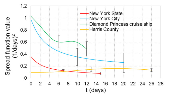
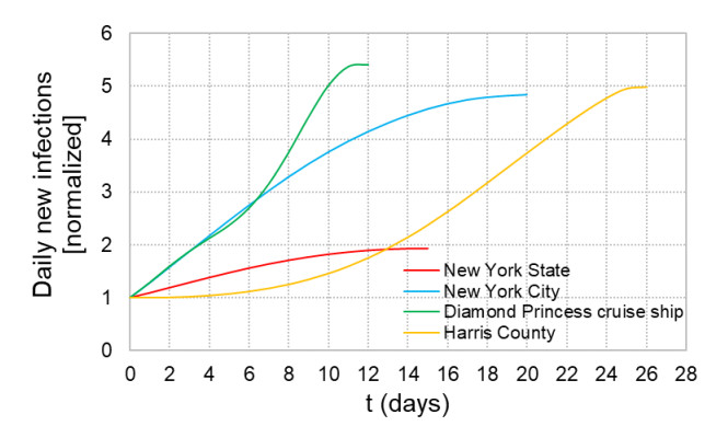
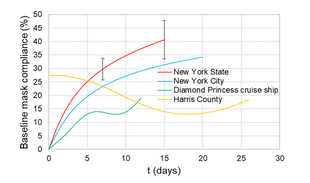
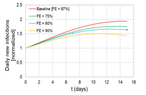
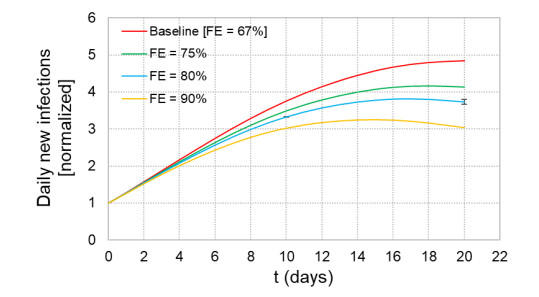
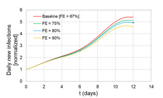
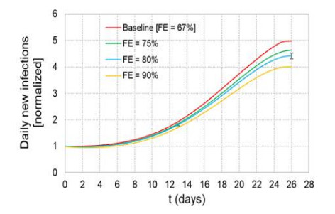
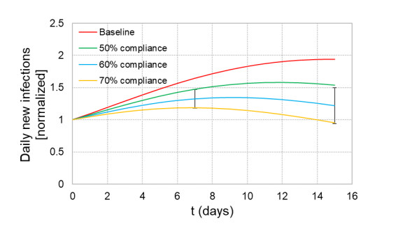
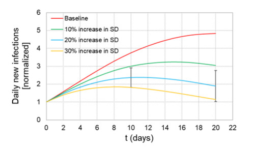
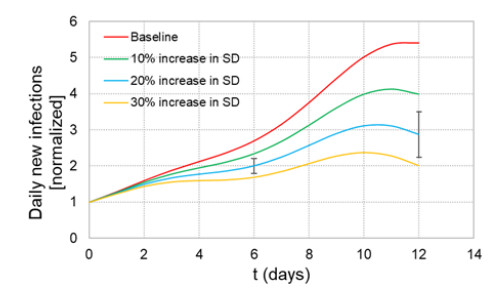
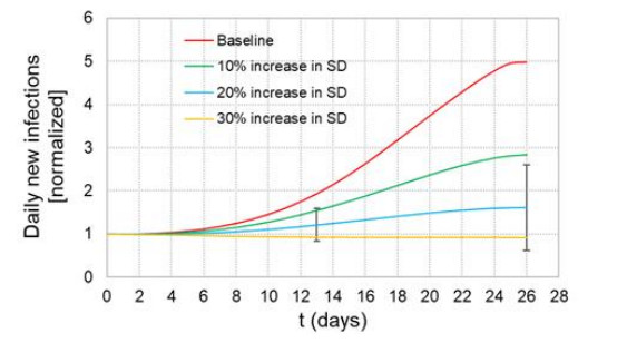
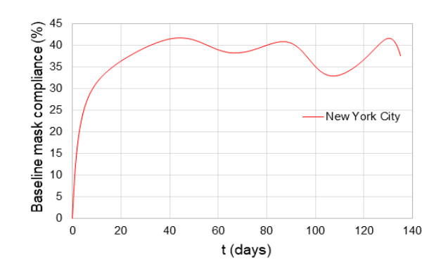
When formulating countermeasures to epidemics such as those generated by COVID-19, estimates of the benefits of a given intervention for a specific population are highly beneficial to policy makers. A recently introduced tool, known as the "dynamic-spread" SIR model, can perform population-specific risk assessment. Behavior is quantified by the dynamic-spread function, which includes the mechanisms of droplet reduction using facemasks and transmission control due to social distancing. The spread function is calibrated using infection data from a previous wave of the infection, or other data felt to accurately represent the population behaviors. The model then computes the rate of spread of the infection for different hypothesized interventions, over the time window for the calibration data. The dynamic-spread model was used to assess the benefit of three enhanced intervention strategies – increased mask filtration efficiency, higher mask compliance, and elevated social distancing – in four COVID-19 scenarios occurring in 2020: the first wave (i.e. until the first peak in numbers of new infections) in New York City; the first wave in New York State; the spread aboard the Diamond Princess Cruise Liner; and the peak occurring after re-opening in Harris County, Texas. Differences in the efficacy of the same intervention in the different scenarios were estimated. As an example, when the average outward filtration efficiency for facemasks worn in New York City was increased from an assumed baseline of 67% to a hypothesized 90%, the calculated peak number of new infections per day decreased by 40%. For the same baseline and hypothesized filtration efficiencies aboard the Diamond Princess Cruise liner, the calculated peak number of new infections per day decreased by about 15%. An important factor contributing to the difference between the two scenarios is the lower mask compliance (derivable from the spread function) aboard the Diamond Princess.
Citation: Gavin D'Souza, Jenna Osborn, Shayna Berman, Matthew Myers. Comparison of effectiveness of enhanced infection countermeasures in different scenarios, using a dynamic-spread-function model[J]. Mathematical Biosciences and Engineering, 2022, 19(9): 9571-9589. doi: 10.3934/mbe.2022445
When formulating countermeasures to epidemics such as those generated by COVID-19, estimates of the benefits of a given intervention for a specific population are highly beneficial to policy makers. A recently introduced tool, known as the "dynamic-spread" SIR model, can perform population-specific risk assessment. Behavior is quantified by the dynamic-spread function, which includes the mechanisms of droplet reduction using facemasks and transmission control due to social distancing. The spread function is calibrated using infection data from a previous wave of the infection, or other data felt to accurately represent the population behaviors. The model then computes the rate of spread of the infection for different hypothesized interventions, over the time window for the calibration data. The dynamic-spread model was used to assess the benefit of three enhanced intervention strategies – increased mask filtration efficiency, higher mask compliance, and elevated social distancing – in four COVID-19 scenarios occurring in 2020: the first wave (i.e. until the first peak in numbers of new infections) in New York City; the first wave in New York State; the spread aboard the Diamond Princess Cruise Liner; and the peak occurring after re-opening in Harris County, Texas. Differences in the efficacy of the same intervention in the different scenarios were estimated. As an example, when the average outward filtration efficiency for facemasks worn in New York City was increased from an assumed baseline of 67% to a hypothesized 90%, the calculated peak number of new infections per day decreased by 40%. For the same baseline and hypothesized filtration efficiencies aboard the Diamond Princess Cruise liner, the calculated peak number of new infections per day decreased by about 15%. An important factor contributing to the difference between the two scenarios is the lower mask compliance (derivable from the spread function) aboard the Diamond Princess.

| [1] |
R. O. J. H. Stutt, R. Retkute, M. Bradley, C. A. Gilligan, J. A. Colvin, Modelling framework to assess the likely effectiveness of facemasks in combination with 'lock-down' in managing the COVID-19 pandemic, Proceed. Royal Soc. A Math. Phys. Eng. Sci., 476 (2020), 20200376. https://doi.org/10.1098/rspa.2020.0376 doi: 10.1098/rspa.2020.0376

|
| [2] |
G. Giordano, F. Blanchini, R. Bruno, P. Colaneri, A. Di Filippo, A. Di Matteo, et al., Modelling the COVID-19 epidemic and implementation of population-wide interventions in Italy, Nat. Med., 26 (2020), 855–860. https://doi.org/10.1038/s41591-020-0883-7 doi: 10.1038/s41591-020-0883-7
|
| [3] |
I. Cooper, A. Mondal, C. Antonopoulos, A SIR model assumption for the spread of COVID-19 in different communities, Chaos Soliton. Fract., 139 (2020), 110057. https://doi.org/10.1016/j.chaos.2020.110057 doi: 10.1016/j.chaos.2020.110057
|
| [4] |
A. L. Bertozzi, E. Franco, G. Mohlerd, M. B. Shorte, D. Sledge, The challenges of modeling and forecasting the spread of COVID-19, Proc. Nat. Acad. Sci., 117 (2020), 16732–16738. https://doi.org/10.1073/pnas.2006520117 doi: 10.1073/pnas.2006520117
|
| [5] |
C. N. Ngonghala, E. Iboi, S. Eikenberry, M. Scotch, C. R. MacIntyre, M. H. Bonds, et al., Mathematical assessment of the impact of non-pharmaceutical interventions on curtailing the 2019 novel Coronavirus, Math. Biosci., 325 (2020), 108364. https://doi.org/10.1016/j.mbs.2020.108364 doi: 10.1016/j.mbs.2020.108364
|
| [6] |
S. E. Eikenberry, M. Mancuso, E. Iboi, T. Phan, K. Eikenberry, Y. Kuang, et al., To mask or not to mask: Modeling the potential for face mask use by the general public to curtail the COVID-19 pandemic, Infect. Disease Model., 5 (2020), 293–308. https://doi.org/10.1016/j.idm.2020.04.001 doi: 10.1016/j.idm.2020.04.001
|
| [7] |
J. Fernández-Villaverde, C. I. Jones, Estimating and simulating a SIRD Model of COVID-19 for many countries, states, and cities, J. Econom. Dynam. Control., (2022), 104318. https://doi.org/10.1016/j.jedc.2022.104318 doi: 10.1016/j.jedc.2022.104318
|
| [8] |
J. Osborn, S. Berman, S. Bender-Bier, G. D'Souza, M. Myers, Retrospective analysis of interventions to epidemics using dynamic simulation of population behavior, Math. Biosci., 341 (2021), 108712. https://doi.org/10.1016/j.mbs.2021.108712 doi: 10.1016/j.mbs.2021.108712
|
| [9] |
N. I. Stilianakis, Y. Drossinos, Dynamics of infectious disease transmission by inhalable respiratory droplets. J. Royal Soc. Interf., 7 (2010), 1355–1366. https://doi.org/10.1098/rsif.2010.0026 doi: 10.1098/rsif.2010.0026
|
| [10] |
M. Myers, J. Yan, P. Hariharan, S. Guha, A mathematical model for assessing the effectiveness of protective devices in reducing risk of infection by inhalable droplets, Math. Med. Biol., 35 (2018), 1–23. https://doi.org/10.1093/imammb/dqw018 doi: 10.1093/imammb/dqw018
|
| [11] |
J. Yan, P. Hariharan, S. Guha, M. Myers, Modeling the effectiveness of respiratory protective devices in reducing influenza outbreak, Risk Analysis, 39 (2019), 647–661. https://doi.org/10.1111/risa.13181 doi: 10.1111/risa.13181
|
| [12] |
F. Zhou, T. Yu, R. Du, G. Fan, Y. Liu, Z. Liu, et al., Clinical course and risk factors for mortality of adult inpatients with COVID-19 in Wuhan, China: A retrospective cohort study, Lancet, 395 (2020), 1054–1062. https://doi.org/10.1016/S0140-6736(20)30566-3 doi: 10.1016/S0140-6736(20)30566-3
|
| [13] | A. Kerr, A Historical Timeline of COVID-19 in New York City, Investopedia, 2021. |
| [14] | C. Francescani, Timeline: The first 100 days of New York Gov. Andrew Cuomo's COVID-19 response, ABC News, 2020. |
| [15] | National Institute of Infectious Diseases, Japan, (2020). https://www.niid.go.jp/niid/en/2019-ncov-e/9407-covid-dp-fe-01.html |
| [16] |
E. Nakazawa, H. Ino, A. Akabayashi, Chronology of COVID-19 cases on the diamond princess cruise ship and ethical considerations: A report from Japan, Disaster Med. Public Health Prep., 14 (2020), 506–513. https://doi.org/10.1017/dmp.2020.50 doi: 10.1017/dmp.2020.50
|
| [17] | Harris County Commissioners Court Agenda, Harris County, Texas, (2020). https://agenda.harriscountytx.gov/COVID19Orders.aspx |
| [18] | Johns Hopkins Coronavirus Resource Center, (2020). https://coronavirus.jhu.edu/map.html |
| [19] | NYC Health, (2020). https://www1.nyc.gov/site/doh/covid/covid-19-data.page |
| [20] | The New York Times, (2020). https://www.nytimes.com/interactive/2020/us/new-york-coronavirus-cases.html |
| [21] |
K. Mizumoto, G. Chowell, Transmission potential of the novel coronavirus (COVID-19) onboard the diamond Princess Cruises Ship, 2020, Infect. Disease Model., 5 (2021), 264–270. https://doi.org/10.1016/j.idm.2020.02.003 doi: 10.1016/j.idm.2020.02.003
|
| [22] | Harris County/City of Houston COVID-19 Data Hub, (2020). https://covid-harriscounty.hub.arcgis.com |
| [23] |
J. Howard, A. Huang, Z. Lik, Z. Tufekci, V. Zdimal, H. M. van der Westhuizen, et al., Face masks against COVID-19: An evidence review, Proc. Nat. Acad. Sci. U.S.A., 118 (2021), e2014564118. https://doi.org/10.1073/pnas.2014564118 doi: 10.1073/pnas.2014564118
|
| [24] | A. Newman, Are New Yorkers wearing masks? Here's what we found in each borough, The New York Times, 2020. https://www.nytimes.com/2020/08/20/nyregion/nyc-face-masks.html |
| [25] | H. Enten, The Northeast leads the country in mask-wearing, CNN, June 26, 2020. https://www.cnn.com/2020/06/26/politics/maskwearing-coronavirus-analysis/index.html |
| [26] | M. Brenan, Americans' Face Mask Usage Varies Greatly by Demographics, Gallup, 2020. https://news.gallup.com/poll/315590/americans-face-mask-usage-varies-greatly-demographics.aspx |
| [27] |
S. Guha, A. Herman, I. A. Carr, D. Porter, R. Natu, S. Berman, et al., Comprehensive characterization of protective face coverings made from household fabrics, PLoS One, 16 (2021), e0244626. https://doi.org/10.1371/journal.pone.0244626 doi: 10.1371/journal.pone.0244626
|
| [28] |
A. R. Ives, C. Bozzuto, Estimating and explaining the spread of COVID-19 at the county level in the USA, Commun. Biol., 4 (2021), 60. https://doi.org/10.1038/s42003-020-01609-6 doi: 10.1038/s42003-020-01609-6
|
| [29] |
S. Zhang, M. Diao, W. Yu, L. Pei, Z. Lin, D. Chen, Estimation of the reproductive number of novel coronavirus (COVID-19) and the probable outbreak size on the Diamond Princess cruise ship: A data-driven analysis, Int. J. Infect. Diseases, 93 (2020), 201–204. https://doi.org/10.1016/j.ijid.2020.02.033 doi: 10.1016/j.ijid.2020.02.033
|
| [30] |
K. T. L. Sy, L. F. White, B. E. Nichols, Population density and basic reproductive number of COVID-19 across United States counties, PLoS One, 16 (2021), e0249271. https://doi.org/10.1371/journal.pone.0249271 doi: 10.1371/journal.pone.0249271
|
| [31] | American Society of Mechanical Engineers, ASME V & V 20-2009 - Standard for Verification and Validation in Computational Fluid Dynamics and Heat Transfer, ASME, New York, 2009. |
Figures(16)

Gavin D'Souza, Jenna Osborn, Shayna Berman, Matthew Myers. Comparison of effectiveness of enhanced infection countermeasures in different scenarios, using a dynamic-spread-function model[J]. Mathematical Biosciences and Engineering, 2022, 19(9): 9571-9589. doi: 10.3934/mbe.2022445


 DownLoad: