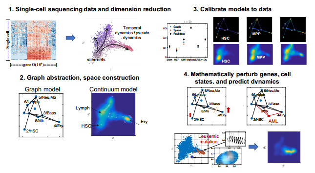
Single-cell sequencing technologies have revolutionized molecular and cellular biology and stimulated the development of computational tools to analyze the data generated from these technology platforms. However, despite the recent explosion of computational analysis tools, relatively few mathematical models have been developed to utilize these data. Here we compare and contrast two cell state geometries for building mathematical models of cell state-transitions with single-cell RNA-sequencing data with hematopoeisis as a model system; (i) by using partial differential equations on a graph representing intermediate cell states between known cell types, and (ii) by using the equations on a multi-dimensional continuous cell state-space. As an application of our approach, we demonstrate how the calibrated models may be used to mathematically perturb normal hematopoeisis to simulate, predict, and study the emergence of novel cell states during the pathogenesis of acute myeloid leukemia. We particularly focus on comparing the strength and weakness of the graph model and multi-dimensional model.
Citation: Heyrim Cho, Ya-Huei Kuo, Russell C. Rockne. Comparison of cell state models derived from single-cell RNA sequencing data: graph versus multi-dimensional space[J]. Mathematical Biosciences and Engineering, 2022, 19(8): 8505-8536. doi: 10.3934/mbe.2022395
Single-cell sequencing technologies have revolutionized molecular and cellular biology and stimulated the development of computational tools to analyze the data generated from these technology platforms. However, despite the recent explosion of computational analysis tools, relatively few mathematical models have been developed to utilize these data. Here we compare and contrast two cell state geometries for building mathematical models of cell state-transitions with single-cell RNA-sequencing data with hematopoeisis as a model system; (i) by using partial differential equations on a graph representing intermediate cell states between known cell types, and (ii) by using the equations on a multi-dimensional continuous cell state-space. As an application of our approach, we demonstrate how the calibrated models may be used to mathematically perturb normal hematopoeisis to simulate, predict, and study the emergence of novel cell states during the pathogenesis of acute myeloid leukemia. We particularly focus on comparing the strength and weakness of the graph model and multi-dimensional model.

| [1] |
V. Svensson, R. Vento-Tormo, S. A. Teichmann, Exponential scaling of single-cell RNA-seq in the past decade, Nat. Protoc., 13 (2018), 599–604. https://doi.org/10.1038/nprot.2017.149 doi: 10.1038/nprot.2017.149

|
| [2] |
G. X. Zheng, J. M. Terry, P. Belgrader, P. Ryvkin, Z. W. Bent, R. Wilson, et al., Massively parallel digital transcriptional profiling of single cells, Nat. Commun., 8 (2017), 14049. http://dx.doi.org/10.1038/ncomms14049 doi: 10.1038/ncomms14049
|
| [3] | T. Stuart, R. Satija, Integrative single-cell analysis, Nat. Rev. Genet., 20 (2019), 257–272. http://www.nature.com/articles/s41576-019-0093-7 |
| [4] |
W. Saelens, R. Cannoodt, H. Todorov, Y. Saeys, A comparison of single-cell trajectory inference methods: towards more accurate and robust tools, Nat. Biotechn., 37 (2019), 547–554. https://doi.org/10.1038/s41587-019-0071-9 doi: 10.1038/s41587-019-0071-9
|
| [5] |
V. Y. Kiselev, T. S. Andrews, M. Hemberg, Challenges in unsupervised clustering of single-cell RNA-seq data, Nat. Rev. Genet., 20 (2019), 273–282. https://doi.org/10.1038/s41576-018-0088-9 doi: 10.1038/s41576-018-0088-9
|
| [6] |
R. D. Brackston, E. Lakatos, M. P. Stumpf, Transition state characteristics during cell differentiation, PLoS Comput. Biol., 14 (2018), e1006405. https://doi.org/10.1371/journal.pcbi.1006405 doi: 10.1371/journal.pcbi.1006405
|
| [7] |
E. Marco, R. L. Karp, G. Guo, P. Robson, A. H. Hart, L. Trippa, et al., Bifurcation analysis of single-cell gene expression data reveals epigenetic landscape, Proc. Nat. Academy Sci., 111 (2014), E5643–E5650. https://doi.org/10.1073/pnas.1408993111 doi: 10.1073/pnas.1408993111
|
| [8] |
A. E. Teschendorff, T. Enver, Single-cell entropy for accurate estimation of differentiation potency from a cell's transcriptome, Nat. Commun., 8 (2017), 15599, http://dx.doi.org/10.1038/ncomms15599. doi: 10.1038/ncomms15599
|
| [9] |
S. Jin, A. L. Maclean, T. Peng, Q. Nie, ScEpath: Energy landscape-based inference of transition probabilities and cellular trajectories from single-cell transcriptomic data, Bioinformatics, 34 (2018), 2077–2086. https://doi.org/10.1093/bioinformatics/bty058 doi: 10.1093/bioinformatics/bty058
|
| [10] |
J. Guo, J. Zheng, HopLand: Single-cell pseudotime recovery using continuous Hopfield network-based modeling of Waddington's epigenetic landscape, Bioinformatics, 33 (2017), i102–i109. https://doi.org/10.1093/bioinformatics/btx232 doi: 10.1093/bioinformatics/btx232
|
| [11] | M. Zwiessele, N. D. Lawrence, Topslam: Waddington Landscape Recovery for Single Cell Experiments, preprint, BioRxiv, 2017: 057778. https://doi.org/10.1101/057778 |
| [12] | H. Cho, K. Ayers, L. DePillis, Y. h. Kuo, J. Park, A. Radunskaya, et al., Modeling acute myeloid leukemia in a continuum of differentiation states, Lett. Biomath., 5 (2018), S69–S98. |
| [13] |
S. Nestorowa, F. K. Hamey, B. Pijuan Sala, E. Diamanti, M. Shepherd, E. Laurenti, et al., A single-cell resolution map of mouse hematopoietic stem and progenitor cell differentiation, Blood, 128 (2016), 20–32. https://doi.org/10.1182/blood-2016-05-716480 doi: 10.1182/blood-2016-05-716480
|
| [14] |
F. Paul, Y. Arkin, A. Giladi, D. A. Jaitin, E. Kenigsberg, H. Keren-Shaul, et al., Transcriptional heterogeneity and lineage commitment in myeloid progenitors, Cell, 163 (2015), 1663–1677. https://doi.org/10.1016/j.cell.2015.11.013 doi: 10.1016/j.cell.2015.11.013
|
| [15] |
L. Haghverdi, F. Buettner, F. Theis, Diffusion maps for high-dimensional single-cell analysis of differentiation data, Bioinformatics, 31 (2015), 2989–2998. https://doi.org/10.1093/bioinformatics/btv325 doi: 10.1093/bioinformatics/btv325
|
| [16] |
M. Barron, J. Li, Identifying and removing the cell-cycle effect from single-cell rna-sequencing data, Sci. Rep., 6 (2016), 33892. https://doi.org/10.1038/srep33892 doi: 10.1038/srep33892
|
| [17] |
J. Wang, L. Xu, E. Wang, Potential landscape and flux framework of nonequilibrium networks: robustness, dissipation, and coherence of biochemical oscillations, Proc. Nat. Acad. Sci., 105 (2008), 12271–12276. https://doi.org/10.1073/pnas.0800579105 doi: 10.1073/pnas.0800579105
|
| [18] |
Z. I. Botev, D. P. Kroese, The generalized cross entropy method, with applications to probability density estimation, Methodol. Comput. Appl. Probab., 13 (2011), 1–27. https://doi.org/10.1007/s11009-009-9133-7 doi: 10.1007/s11009-009-9133-7
|
| [19] |
M. Doumic, A. Marciniak-Czochra, B. Perthame, J. P. Zubelli, A structured population model of cell differentiation, SIAM J. Appl. Math., 71 (2011), 1918–1940. https://doi.org/10.1137/100816584 doi: 10.1137/100816584
|
| [20] |
C. Weinreb, S. Wolock, B. K. Tusi, M. Socolovsky, A. M. Klein, Fundamental limits on dynamic inference from single-cell snapshots, Proc. Nat. Acad. Sci., 115 (2018), E2467–E2476. https://doi.org/10.1073/pnas.1714723115 doi: 10.1073/pnas.1714723115
|
| [21] |
G. H. T. Yeo, S. D. Saksena, D. K. Gifford, Generative modeling of single-cell time series with prescient enables prediction of cell trajectories with interventions, Nat. Commun., 12 (2021), 3222. https://doi.org/10.1038/s41467-021-23518-w doi: 10.1038/s41467-021-23518-w
|
| [22] | L. C. Evans, An Introduction to Stochastic Differential Equations, American Mathematical Society, 2014. |
| [23] |
F. A. Wolf, F. K. Hamey, M. Plass, J. Solana, J. S. Dahlin, B. Göttgens, et al., PAGA: Graph abstraction reconciles clustering with trajectory inference through a topology preserving map of single cells, Genome Biol., 20 (2019), 59. https://doi.org/10.1186/s13059-019-1663-x doi: 10.1186/s13059-019-1663-x
|
| [24] | L. C. Evans, Partial Differential Equations, 2nd edition, American Mathematical Society, 2010. |
| [25] |
R. C. Rockne, S. Branciamore, J. Qi, D. E. Frankhouser, D. O'Meally, W. K. Hua, et al., State-transition analysis of time-sequential gene expression identifies critical points that predict development of acute myeloid leukemia, Cancer Res., 80 (2020), 3157–3169. https://doi.org/10.1158/0008-5472.CAN-20-0354 doi: 10.1158/0008-5472.CAN-20-0354
|
| [26] | A. W. Bowman, A. Azzalini, Applied Smoothing Techniques for Data Analysis, Oxford University Press Inc., New York, 1997. |
| [27] |
Q. Cai, R. Jeannet, W. K. K. Hua, G. J. Cook, B. Zhang, J. Qi, et al., Cbf$\beta$-smmhc creates aberrant megakaryocyte-erythroid progenitors prone to leukemia initiation in mice, Blood, 128 (2016), 1503–1515. https://doi.org/10.1182/blood-2016-01-693119 doi: 10.1182/blood-2016-01-693119
|
| [28] |
P. Liu, S. A. Tarlé, A. Hajra, D. F. Claxton, P. Marlton, M. Freedman, et al., Fusion between transcription factor cbf beta/pebp2 beta and a myosin heavy chain in acute myeloid leukemia, Science, 261 (1993), 1041–1044. https://doi.org/10.1126/science.8351518 doi: 10.1126/science.8351518
|
| [29] |
P. P. Liu, C. Wijmenga, A. Hajra, T. B. Blake, C. A. Kelley, R. S. Adelstein, et al., Identification of the chimeric protein product of the cbfb-myh11 fusion gene in inv(16) leukemia cells, Genes Chromosomes Cancer, 16 (1996), 77–87. https://doi.org/10.1002/(SICI)1098-2264(199606)16:2<77::AID-GCC1>3.0.CO;2-%23 doi: 10.1002/(SICI)1098-2264(199606)16:2<77::AID-GCC1>3.0.CO;2-%23
|
| [30] |
L. H. Castilla, L. Garrett, N. Adya, D. Orlic, A. Dutra, S. Anderson, et al., The fusion gene cbfb-myh11 blocks myeloid differentiation and predisposes mice to acute myelomonocytic leukaemia, Nat. Genet., 23 (1999), 144–146. https://doi.org/10.1038/13776 doi: 10.1038/13776
|
| [31] |
Y. H. H. Kuo, S. F. Landrette, S. A. Heilman, P. N. Perrat, L. Garrett, P. P. Liu, et al., Cbf$\beta$-smmhc induces distinct abnormal myeloid progenitors able to develop acute myeloid leukemia, Cancer Cell, 9 (2006), 57–68. https://doi.org/10.1016/j.ccr.2005.12.014 doi: 10.1016/j.ccr.2005.12.014
|
| [32] |
Y. H. H. Kuo, R. M. Gerstein, L. H. Castilla, Cbf$\beta$-smmhc impairs differentiation of common lymphoid progenitors and reveals an essential role for runx in early b-cell development, Blood, 111 (2008), 1543–1551. https://doi.org/10.1182/blood-2007-07-104422 doi: 10.1182/blood-2007-07-104422
|
| [33] |
C. J. H. Pronk, D. J. Rossi, R. Mansson, J. L. Attema, G. L. Norddahl, C. K. F. Chan, et al., Elucidation of the phenotypic, functional, and molecular topography of a myeloerythroid progenitor cell hierarchy, Cell Stem Cell, 1 (2007), 428–442. https://doi.org/10.1016/j.stem.2007.07.005 doi: 10.1016/j.stem.2007.07.005
|
| [34] |
K. Akashi, D. Traver, T. Miyamoto, I. L. Weissman, A clonogenic common myeloid progenitor that gives rise to all myeloid lineages, Nature, 404 (2000), 193–197. https://doi.org/10.1038/35004599 doi: 10.1038/35004599
|
| [35] |
S. Ng, A. Mitchell, J. A. Kennedy, W. C. Chen, J. Mcleod, N. Ibrahimova, et al., A 17-gene stemness score for rapid determination of risk in acute leukaemia, Nature, 540 (2016), 433–437, http://dx.doi.org/10.1038/nature20598 doi: 10.1038/nature20598
|
| [36] |
C. Pabst, A. Bergeron, V. P. Lavall, J. Yeh, P. Gendron, G. L. Norddahl, et al., GPR56 identifies primary human acute myeloid leukemia cells with high repopulating potential in vivo, Blood, 127 (2017), 2018–2027. https://doi.org/10.1182/blood-2015-11-683649 doi: 10.1182/blood-2015-11-683649
|
| [37] |
T. D. Sherman, L. T. Kagohara, R. Cao, R. Cheng, M. Satriano, M. Considine, et al., CancerInSilico: An R/Bioconductor package for combining mathematical and statistical modeling to simulate time course bulk and single cell gene expression data in cancer, PLOS Comput. Biol., 14 (2019), e1006935. https://doi.org/10.1371/journal.pcbi.1006935 doi: 10.1371/journal.pcbi.1006935
|
| [38] |
M. C. Ferrall-Fairbanks, M. Ball, E. Padron, P. M. Altrock, Leveraging single cell RNA sequencing experiments to model intra-tumor heterogeneity, Clin. Cancer Inf., 3 (2019), 1–10. http://doi.org/10.1200/CCI.18.00074 doi: 10.1200/CCI.18.00074
|
| [39] |
E. Papalexi, R. Satija, Single-cell RNA sequencing to explore immune cell heterogeneity, Nat. Rev. Immunol., 18 (2018), 35–45. https://doi.org/10.1038/nri.2017.76. doi: 10.1038/nri.2017.76
|
| [40] |
G. Schiebinger, J. Shu, R. Jaenisch, A. Regev, E. S. Lander, Optimal-transport analysis of single-cell gene expression identifies developmental trajectories in reprogramming, Cell, 176 (2019), 928–943. https://doi.org/10.1016/j.cell.2019.01.006. doi: 10.1016/j.cell.2019.01.006
|
| [41] |
G. Schiebinger, Reconstructing developmental landscapes and trajectories from single-cell data, Curr. Opin. Syst. Biol., 27 (2021), 100351. https://doi.org/10.1016/j.coisb.2021.06.002 doi: 10.1016/j.coisb.2021.06.002
|
| [42] |
M. Setty, V. Kiseliovas, J. Levine, A. Gayoso, L. Mazutis, D. Pe'er, Characterization of cell fate probabilities in single-cell data with Palantir, Nat. Biotechnol., 37 (2019), 451–460, http://dx.doi.org/10.1038/s41587-019-0068-4 doi: 10.1038/s41587-019-0068-4
|
| [43] |
S. Hormoz, Z. S. Singer, J. M. Linton, Y. E. Antebi, B. I. Shraiman, M. B. Elowitz, Inferring cell-state transition dynamics from lineage trees and endpoint single-cell measurements, Cell Syst., 3 (2016), 419–433. https://doi.org/10.1016/j.cels.2016.10.015 doi: 10.1016/j.cels.2016.10.015
|
| [44] |
D. S. Fischer, A. K. Fiedler, E. M. Kernfeld, R. M. J. Genga, A. Bastidas-ponce, M. Bakhti, et al., Inferring population dynamics from single-cell RNA-sequencing time series data, Nat. Biotechnol., 37 (2019), 461–468. https://doi.org/10.1038/s41587-019-0088-0. doi: 10.1038/s41587-019-0088-0
|
| [45] |
Q. Jiang, S. Zhang, L. Wan, Dynamic inference of cell developmental complex energy landscape from time series single-cell transcriptomic data, PLOS Comput. Biol., 18 (2022), e1009821. https://doi.org/10.1371/journal.pcbi.1009821 doi: 10.1371/journal.pcbi.1009821
|
| [46] | A. Sharma, E. Y. Cao, V. Kumar, X. Zhang, H. S. Leong, A. M. L. Wong, et al., Longitudinal single-cell RNA sequencing of patient-derived primary cells reveals drug-induced infidelity in stem cell hierarchy, Nat. Commun., https://doi.org/10.1038/s41467-018-07261-3. |
| [47] |
M. Karaayvaz, S. Cristea, S. M. Gillespie, A. P. Patel, R. Mylvaganam, C. C. Luo, et al., Unravelling subclonal heterogeneity and aggressive disease states in TNBC through single-cell RNA-seq, Nat. Commun., 9 (2018), 3588. https://doi.org/10.1038/s41467-018-06052-0. doi: 10.1038/s41467-018-06052-0
|
| [48] |
G. La Manno, R. Soldatov, A. Zeisel, E. Braun, H. Hochgerner, V. Petukhov, et al., RNA velocity of single cells, Nature, 560 (2018), 494–498. https://doi.org/10.1038/s41586-018-0414-6 doi: 10.1038/s41586-018-0414-6
|
| [49] | G. Eraslan, Ž. Avsec, J. Gagneur, F. J. Theis, Deep learning : new computational modelling techniques for genomics, Nat. Rev. Genet., 20 (2019). https://doi.org/10.1038/s41576-019-0122-6 |
| [50] |
N. Gaw, A. Hawkins-Daarud, L. S. Hu, H. Yoon, L. Wang, Y. Xu, et al., Integration of machine learning and mechanistic models accurately predicts variation in cell density of glioblastoma using multiparametric MRI, Sci. Rep., 9 (2019), 10063. https://doi.org/10.1038/s41598-019-46296-4 doi: 10.1038/s41598-019-46296-4
|
| [51] |
R. C. Rockne, A. Hawkins-Daarud, K. R. Swanson, J. P. Sluka, J. A. Glazier, P. Macklin, et al., The 2019 mathematical oncology roadmap, Phys. Biol., 16 (2019), 4. https://doi.org/10.1088/1478-3975/ab1a09 doi: 10.1088/1478-3975/ab1a09
|
| [52] |
X. Qiu, Y. Zhang, J. D. Martin-Rufino, C. Weng, S. Hosseinzadeh, D. Yang, et al., Mapping transcriptomic vector fields of single cells, Cell, 185 (2022), 690–711. https://doi.org/10.1016/j.cell.2021.12.045 doi: 10.1016/j.cell.2021.12.045
|
| [53] |
S. K. Chu, S. Zhao, Y. Shyr, Q. Liu, Comprehensive evaluation of noise reduction methods for single-cell rna sequencing data, Briefings Bioinf., 23 (2022), bbab565. https://doi.org/10.1093/bib/bbab565 doi: 10.1093/bib/bbab565
|
| [54] |
M. Mojtahedi, A. Skupin, J. Zhou, I. G. Castaño, R. Y. Leong-Quong, H. Chang, et al., Cell fate decision as high-dimensional critical state transition, PLoS Biol., 14 (2016), 1–28. https://doi.org/10.1371/journal.pbio.2000640 doi: 10.1371/journal.pbio.2000640
|
| [55] |
C. Li, L. Zhang, Q. Nie, Landscape reveals critical network structures for sharpening gene expression boundaries, BMC Syst. Biol., 12 (2018), 67. https://doi.org/10.1186/s12918-018-0595-5 doi: 10.1186/s12918-018-0595-5
|
| [56] |
J. I. Joo, J. X. Zhou, S. Huang, K. H. Cho, Determining relative dynamic stability of cell states using boolean network model, Sci. Rep., 8 (2018), 12077. https://doi.org/10.1038/s41598-018-30544-0 doi: 10.1038/s41598-018-30544-0
|
| [57] |
B. E. Shepherd, P. Guttorp, P. M. Lansdorp, J. L. Abkowitz, Estimating human hematopoietic stem cell kinetics using granulocyte telomere lengths, Exp. Hematol., 32 (2004), 1040–1050. https://doi.org/10.1016/j.exphem.2004.07.023 doi: 10.1016/j.exphem.2004.07.023
|
| [58] | E. P. Cronkite, Kinetics of granulopoiesis, Clin. Haematol., 8 (1979), 351–370. |
| [59] |
S. Hao, C. Chen, T. Cheng, Cell cycle regulation of hematopoietic stem or progenitor cells, Int. J. Hematol., 103 (2016), 487–497. https://doi.org/10.1007/s12185-016-1984-4 doi: 10.1007/s12185-016-1984-4
|
| [60] |
E. M. Pietras, M. R. Warr, E. Passegué, Cell cycle regulation in hematopoietic stem cells, J. Cell Biol., 195 (2011), 709–720. https://doi.org/10.1083/jcb.201102131 doi: 10.1083/jcb.201102131
|
| [61] |
T. Stiehl, A. D. Ho, A. Marciniak-Czochra, The impact of CD34+ cell dose on engraftment after SCTs: personalized estimates based on mathematical modeling, Bone Marrow Transp., 49 (2014), 30–37. https://doi.org/10.1038/bmt.2013.138 doi: 10.1038/bmt.2013.138
|
| [62] |
R. R. Coifman, S. Lafon, A. B. Lee, M. Maggioni, B. Nadler, F. Warner, et al., Geometric diffusions as a tool for harmonic analysis and structure definition of data : Diffusion maps, Proc. Natl. Acad. Sci., 102 (2005), 7426–7431. https://doi.org/10.1073/pnas.0500334102 doi: 10.1073/pnas.0500334102
|
| [63] |
L. Haghverdi, M. Büttner, F. Wolf, F. Buettner, F. Theis, Diffusion pseudotime robustly reconstructs lineage branching, Nat. Methods, 13 (2016), 845–848. https://doi.org/10.1038/nmeth.3971 doi: 10.1038/nmeth.3971
|
| [64] |
M. Jacomy, T. Venturini, S. Heymann, M. Bastian, Forceatlas2, a continuous graph layout algorithm for handy network visualization designed for the gephi software, PLOS One, 9 (2014), e98679. https://doi.org/10.1371/journal.pone.0098679 doi: 10.1371/journal.pone.0098679
|
Figures(15) / Tables(4)

Heyrim Cho, Ya-Huei Kuo, Russell C. Rockne. Comparison of cell state models derived from single-cell RNA sequencing data: graph versus multi-dimensional space[J]. Mathematical Biosciences and Engineering, 2022, 19(8): 8505-8536. doi: 10.3934/mbe.2022395


 DownLoad: