Stability analysis and optimal control of a rumor propagation model based on two communication modes: friends and marketing account pushing

Ying Yu; Jiaomin Liu; Jiadong Ren; Cuiyi Xiao; Ying Yu; Jiaomin Liu; Jiadong Ren; Cuiyi Xiao

doi:10.3934/mbe.2022204

Mathematical Biosciences and Engineering

2022, Volume 19, Issue 5: 4407-4428. doi: 10.3934/mbe.2022204

Previous Article Next Article

Research article Special Issues

Stability analysis and optimal control of a rumor propagation model based on two communication modes: friends and marketing account pushing

1.
College of Information Science and Engineering, Yanshan University, Qinhuangdao, Hebei, China
2.
Liren College of Yanshan University, Qinhuangdao, Hebei, China
3.
Computer Virtual Technology and System Integration Laboratory of Hebei Province, China
4.
College of Mathematics and Information Technology, Hebei Normal University of Science and Technology, Qinhuangdao, Hebei, China

Academic Editor: Cristiana J. Silva

Received: 28 November 2021 Revised: 15 February 2022 Accepted: 17 February 2022 Published: 02 March 2022

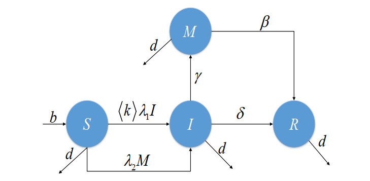
In addition to spreading information among friends, information can also be pushed through marketing accounts to non-friends. Based on these two information dissemination channels, this paper establishes a Susceptible-Infection-Marketing-Removed (SIMR) rumor propagation model. First, we obtain the basic reproduction number $ R_0 $ through the next generation matrix. Second, we prove that the solutions of the model are uniformly bounded and discuss asymptotically stable of the rumor-free equilibrium point and the rumor-prevailing equilibrium point. Third, we propose an optimal control strategy for rumors to control the spread of rumors in the network. Finally, the above theories are verified by numerical simulation methods and the necessary conclusions are drawn.
- rumor propagation model,
- basic reproduction number,
- stability analysis,
- optimal control problem,
- optimization strategy
Citation: Ying Yu, Jiaomin Liu, Jiadong Ren, Cuiyi Xiao. Stability analysis and optimal control of a rumor propagation model based on two communication modes: friends and marketing account pushing[J]. Mathematical Biosciences and Engineering, 2022, 19(5): 4407-4428. doi: 10.3934/mbe.2022204

Related Papers:

Abstract

In addition to spreading information among friends, information can also be pushed through marketing accounts to non-friends. Based on these two information dissemination channels, this paper establishes a Susceptible-Infection-Marketing-Removed (SIMR) rumor propagation model. First, we obtain the basic reproduction number $ R_0 $ through the next generation matrix. Second, we prove that the solutions of the model are uniformly bounded and discuss asymptotically stable of the rumor-free equilibrium point and the rumor-prevailing equilibrium point. Third, we propose an optimal control strategy for rumors to control the spread of rumors in the network. Finally, the above theories are verified by numerical simulation methods and the necessary conclusions are drawn.

References

[1]	R. K. Garrett, Troubling consequences of online political rumoring, Hum. Commun. Res., 37 (2011), 255–274. https://doi.org/10.1111/j.1468-2958.2010.01401.x doi: 10.1111/j.1468-2958.2010.01401.x
[2]	L. Zhu, G. Guan, Dynamical analysis of a rumor spreading model with self-discrimination and time delay in complex networks, Physica A, 533, (2019). https://doi.org/10.1016/j.physa.2019.121953
[3]	L. Zhu, M. Liu, Y. Li, The dynamics analysis of a rumor propagation model in online social networks, Physica A, 520 (2019), 118–137. https://doi.org/10.1016/j.physa.2019.01.013 doi: 10.1016/j.physa.2019.01.013
[4]	H. Sun, Y. Sheng, Q. Cui, An uncertain SIR rumor spreading model, Adv. Differ. Equations, 2021 (2021). https://doi.org/10.1186/s13662-021-03386-w
[5]	L. Zhu, L. Li, Dynamic analysis of rumor-spread-delaying model based on rumor-refuting mechanism, Acta Phys. Sin., 69 (2020), 020501. https://doi.org/10.7498/aps.69.20191503 doi: 10.7498/aps.69.20191503
[6]	L. Zhu, F. Yang, G. Guan, Z. Zhang, Modeling the dynamics of rumor diffusion over complex networks, Inf. Sci., 562 (2021). https://doi.org/10.1016/j.ins.2020.12.071
[7]	R. Li, Y. Li, Z. Meng, Y. Song, G. Jiang, Rumor spreading model considering individual activity and refutation mechanism simultaneously, IEEE Access, 8 (2020), 63065–63076. https://doi.org/10.1109/ACCESS.2020.2983249 doi: 10.1109/ACCESS.2020.2983249
[8]	G. Chen, ILSCR rumor spreading model to discuss the control of rumor spreading in emergency, Physica A, 522 (2019), 88–97. https://doi.org/10.1016/j.physa.2018.11.068 doi: 10.1016/j.physa.2018.11.068
[9]	Z. He, Z. Cai, J. Yu, X. Wang, Y. Sun, Y. Li, Cost-efficient strategies for restraining rumor spreading in mobile social networks, IEEE Trans. Veh. Technol., 66 (2017), 2789–2800. https://doi.org/10.1109/TVT.2016.2585591 doi: 10.1109/TVT.2016.2585591
[10]	J. Chen, L. Yang, X. Yang, Y. Tang, Cost-effective anti-rumor message-pushing schemes, Physica A, 540 (2020), 123085. https://doi.org/10.1016/j.physa.2019.123085 doi: 10.1016/j.physa.2019.123085
[11]	L. Ding, P. Hu, Z. Guan, An efficient hybrid control strategy for restraining rumor spreading, IEEE Trans. Syst. Man Cybern.: Syst., 51 (2021), 6779–6791. https://doi.org/10.1109/TSMC.2019.2963418 doi: 10.1109/TSMC.2019.2963418
[12]	L. Zhu, M. Zhou, Z. Zhang, Dynamical analysis and control strategies of rumor spreading models in both homogeneous and heterogeneous networks, J. Nonlinear Sci., 30 (2020) 2545–2576. https://doi.org/10.1007/s00332-020-09629-6
[13]	S. Chen, H. Jiang, L. Li, J. Li, Dynamical behaviors and optimal control of rumor propagation model with saturation incidence on heterogeneous networks, Chaos, Solitons Fractals, 140 (2020), 110206. https://doi.org/10.1016/j.chaos.2020.110206 doi: 10.1016/j.chaos.2020.110206
[14]	D. Daley, D. Kendall, Epidemics and rumours, Nature, 204 (1964), 1118. https://doi.org/10.1038/2041118a0
[15]	D. Daley, D. Kendall, Stochastic rumours, J. Appl. Math., 1 (1965), 42–55. https://doi.org/10.1093/imamat/1.1.42
[16]	D. Zanette, H. Damián, Dynamics of rumor propagation on small-world networks, Phys. Rev. E Stat. Nonlin. Soft Matter Phys., 65 (2001), 041908. https://doi.org/10.1103/PhysRevE.65.041908 doi: 10.1103/PhysRevE.65.041908
[17]	D. Zanette, Critical behavior of propagation on small-world network, Phys. Rev. E, 64 (2001), 050901. https://doi.org/10.1103/PhysRevE.64.050901 doi: 10.1103/PhysRevE.64.050901
[18]	Y. Moreno, M. Nekovee, Dynamics of rumor spreading in complex networks, Phys. Rev. E, 69 (2004), 066130. https://doi.org/10.1103/PhysRevE.69.066130 doi: 10.1103/PhysRevE.69.066130
[19]	Y. Wang, J. Cao, Z. Jin, H. Zhang, G. Sun, Impact of media coverage on epidemic spreading in complex networks, Physica A, 392 (2013), 5824–5835. https://doi.org/10.1016/j.physa.2013.07.067 doi: 10.1016/j.physa.2013.07.067
[20]	L. Zheng, L. Tang, A node-based SIRS epidemic model with infective media on complex networks, Complexity, 2019 (2019), 1–14. https://doi.org/10.1155/2019/2849196 doi: 10.1155/2019/2849196
[21]	L. Xia, G. Jiang, B. Song, Y. Song, Rumor spreading model considering hesitating mechanism in complex social networks, Physica A, 437 (2015), 295–303. https://doi.org/10.1016/j.physa.2015.05.113 doi: 10.1016/j.physa.2015.05.113
[22]	Q. Liu, T. Li, M. Sun, The analysis of an SEIR rumor propagation model on heterogeneous network, Physica A, 469 (2017), 372–380. https://doi.org/10.1016/j.physa.2016.11.067 doi: 10.1016/j.physa.2016.11.067
[23]	H. Zhu, J. Ma, Analysis of SHIR rumor propagation in random heterogeneous networks with dynamic friendships, Physica A, 513 (2019), 257–271. https://doi.org/10.1016/j.physa.2018.09.015 doi: 10.1016/j.physa.2018.09.015
[24]	Y. Zhang, J. Zhu, Stability analysis of I2S2R rumor spreading model in complex networks, Physica A, 503 (2018), 862–881. https://doi.org/10.1016/j.physa.2018.02.087 doi: 10.1016/j.physa.2018.02.087
[25]	D. Yang, T. Chow, L. Zhong, Q. Zhang, The competitive information spreading over multiplex social networks, Physica A, 503 (2018), 981–990. https://doi.org/10.1016/j.physa.2018.08.096 doi: 10.1016/j.physa.2018.08.096
[26]	W. Liu, T. Li, X. Cheng, H. Xu, X. Liu, Spreading dynamics of a cyber violence model on scale-free networks, AIMS Math., 531 (2019), 121752. https://doi.org/10.1016/j.physa.2019.121752 doi: 10.1016/j.physa.2019.121752
[27]	Y. Yu, J. Liu, J. Ren, Q. Wang, C. Xiao, Minimize the impact of rumors by optimizing the control of comments on the complex network, AIMS Math., 6 (2021), 6140–6159. https://doi.org/10.3934/math.2021360 doi: 10.3934/math.2021360
[28]	P. van den Driessche, J. Watmough, Reproduction numbers and sub-threshold endemic equilibria for compartmental models of diseases transmission, Math. Biosci., 180 (2002), 29–48. https://doi.org/10.1016/S0025-5564(02)00108-6 doi: 10.1016/S0025-5564(02)00108-6
[29]	O. Diekmann, J. Heesterbeek, J. Metz, On the definition and the computation of the basic reproduction ratio R0 in models for infectious diseases in heterogeneous populations, J. Math. Biol., 28 (1990), 365–382. https://doi.org/10.1007/BF00178324 doi: 10.1007/BF00178324
[30]	C. Barril, A. Calsina, J. Ripoll, A practical approach to $R_0$ in continuous-time ecological models, Math. Methods Appl. Sci., 41 (2017), 8432–8445. https://doi.org/10.1002/mma.4673 doi: 10.1002/mma.4673
[31]	D. Breda, F. Florian, J. Ripoll, R. Vermiglio, Efficient numerical computation of the basic reproduction number for structured populations, J. Comput. Appl. Math., 384 (2021), 113165. https://doi.org/10.1016/j.cam.2020.113165 doi: 10.1016/j.cam.2020.113165
[32]	E. X. Dejesus, C. Kaufman, Routh-Hurwitz criterion in the examination of eigenvalues of a system of nonlinear ordinary differential equations, Phys. Rev. A, 35 (1987), 5288. https://doi.org/10.1103/PhysRevA.35.5288 doi: 10.1103/PhysRevA.35.5288
[33]	C. Castillo-Chavez, S. Blower, P. van den Driessche, D. Kirschner, A. A. Yakubu, Mathematical Approaches for Emerging and Re-Emerging Infectious Diseases: An Introduction, Springer, New York, 2002. https://doi.org/10.1007/978-1-4613-0065-6
[34]	E. M. Stein, R. Shakarchi, Real Analysis: Measure Theory, Integration, and Hilbert Spaces, Princeton University Press, 2005. Available from: https://www.academia.edu/25753953/Real_Analysis_Measure_Theory_Integration_and_Hilbert_Spaces_2005_.
[35]	L. Pontryagin, V. Boltyanskii, R. Gamkrelidze, E. Mishchenko, The Mathematical Theory of Optimal Processes, John Wiley & Sons, Inc, 1962. https://doi.org/28812407712881241344
[36]	L. Zhao, W. Qin, J. Cheng, Y. Chen, J. Wang, H. Wei, Rumor spreading model with consideration of forgetting mechanism: A case of online blogging livejournal, Physica A, 390 (2011), 2619–2625. https://doi.org/10.1016/j.physa.2011.03.010 doi: 10.1016/j.physa.2011.03.010
[37]	L. Zhao, H. Cui, X. Qiu, X. Wang, J. Wang, Sir rumor spreading model in the new media age, Physica A, 392 (2013). https://doi.org/10.1016/j.physa.2012.09.030

Reader Comments

Your name:*

Email:*
© 2022 the Author(s), licensee AIMS Press. This is an open access article distributed under the terms of the Creative Commons Attribution License (http://creativecommons.org/licenses/by/4.0)