Facial feature point recognition method for human motion image using GNN

Qingwei Wang; Xiaolong Zhang; Xiaofeng Li; Qingwei Wang; Xiaolong Zhang; Xiaofeng Li

doi:10.3934/mbe.2022175

Mathematical Biosciences and Engineering

2022, Volume 19, Issue 4: 3803-3819. doi: 10.3934/mbe.2022175

Previous Article Next Article

Research article Special Issues

Facial feature point recognition method for human motion image using GNN

1.
Harbin Huade University, Harbin 150025, China
2.
Northeast Forestry University, Harbin 150040, China
3.
Department of Information Engineering, Heilongjiang International University, Harbin 150025, China
academic editor:Weizheng Wang

Received: 29 September 2021 Revised: 14 January 2022 Accepted: 24 January 2022 Published: 10 February 2022

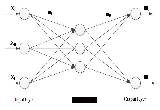
To address the problems of facial feature point recognition clarity and recognition efficiency in different human motion conditions, a facial feature point recognition method using Genetic Neural Network (GNN) algorithm was proposed. As the technical platform, weoll be using the Hikey960 development board. The optimized BP neural network algorithm is used to collect and classify human motion facial images, and the genetic algorithm is introduced into neural network algorithm to train human motion facial images. Combined with the improved GNN algorithm, the facial feature points are detected by the dynamic transplantation of facial feature points, and the detected facial feature points are transferred to the face alignment algorithm to realize facial feature point recognition. The results show that the efficiency and accuracy of facial feature point recognition in different human motion images are higher than 85% and the performance of anti-noise is good, the average recall rate is about 90% and the time-consuming is short. It shows that the proposed method has a certain reference value in the field of human motion image recognition.
- Genetic Neural Network,
- human motion,
- facial feature points,
- facial detection,
- BP neural network
Citation: Qingwei Wang, Xiaolong Zhang, Xiaofeng Li. Facial feature point recognition method for human motion image using GNN[J]. Mathematical Biosciences and Engineering, 2022, 19(4): 3803-3819. doi: 10.3934/mbe.2022175

Related Papers:

Abstract

To address the problems of facial feature point recognition clarity and recognition efficiency in different human motion conditions, a facial feature point recognition method using Genetic Neural Network (GNN) algorithm was proposed. As the technical platform, weoll be using the Hikey960 development board. The optimized BP neural network algorithm is used to collect and classify human motion facial images, and the genetic algorithm is introduced into neural network algorithm to train human motion facial images. Combined with the improved GNN algorithm, the facial feature points are detected by the dynamic transplantation of facial feature points, and the detected facial feature points are transferred to the face alignment algorithm to realize facial feature point recognition. The results show that the efficiency and accuracy of facial feature point recognition in different human motion images are higher than 85% and the performance of anti-noise is good, the average recall rate is about 90% and the time-consuming is short. It shows that the proposed method has a certain reference value in the field of human motion image recognition.

References

[1]	Z. Xu, B. Li, M. Geng, Y. Yuan, AnchorFace: An anchor-based facial landmark detector across large poses, preprint, arXiv: 2007.03221.
[2]	P. Gao, K. Lu, J. Xue, J. Lyu, L. Shao, A facial landmark detection method based on deep knowledge transfer, IEEE Trans. Neural Networks Learn. Syst., 2021. https://doi.org/10.1109/TNNLS.2021.3105247 doi: 10.1109/TNNLS.2021.3105247
[3]	B. Guo, F. Da, Expression-invariant 3D face recognition based on local descriptors, J. Comput. - Aided Des. Comput. Graphics, 31 (2019), 1086–1094. https://doi.org/10.3724/SP.J.1089.2019.17433 doi: 10.3724/SP.J.1089.2019.17433
[4]	D. Wu, X. Jing, L. Zhang, W. Wang, Face recognition with Gabor feature based on Laplacian Pyramid, J. Comput. Appl., z2 (2017), 63–66.
[5]	Y. Guo, E. She, Q. Wang, Z. Li, Face point cloud registration based on improved surf algorithm, Opt. Technol., 44 (2018), 333–338. https://doi.org/10.13741/j.cnki.11-1879/o4.2018.03.014 doi: 10.13741/j.cnki.11-1879/o4.2018.03.014
[6]	J. Xu, Z. Wu, Y. Xu, J. Zeng, Face recognition based on PCA, LDA and SVM, Comput. Eng. Appl., 55 (2019), 34–37. https://doi.org/10.3778/j.issn.1002-8331.1903-0286 doi: 10.3778/j.issn.1002-8331.1903-0286
[7]	T. Liu, X. Zhou, X. Yan, LDA facial expression recognition algorithm combining optical flow characteristics with Gaussian, Comput. Sci., 45 (2018), 286–290.
[8]	L. Sun, C. Zhao, Z. Yan, P. Liu, T. Duckett, R. Stolkin, A novel weakly-supervised approach for RGB-D-based nuclear waste object detection, IEEE Sens. J., 19 (2019), 3487–3500. https://doi.org/10.1109/JSEN.2018.2888815 doi: 10.1109/JSEN.2018.2888815
[9]	P. Liu, H. Yu, S. Cang, Adaptive neural network tracking control for underactuated systems with matched and mismatched disturbances, Nonlinear Dyn., 98 (2019), 1447–1464. https://doi.org/10.1007/s11071-019-05170-8 doi: 10.1007/s11071-019-05170-8
[10]	Z. Tang, H. Yu, C. Lu, P. Liu, X. Jin, Single-trial classification of different movements on one arm based on ERD/ERS and corticomuscular coherence, IEEE Access, 7 (2019), 128185–128197. https://doi.org/10.1109/ACCESS.2019.2940034 doi: 10.1109/ACCESS.2019.2940034
[11]	Z. Tang, C. Li, J. Wu, P. Liu, S. Cheng, Classification of EEG-based single-trial motor imagery tasks using a B-CSP method for BCI, Front. Inf. Technol. Electronic Eng., 20 (2019), 1087–1098. https://doi.org/10.1631/FITEE.1800083 doi: 10.1631/FITEE.1800083
[12]	H. Xiong, C. Jin, M. Alazab, K. Yeh, H. Wang, T. R. R. Gadekallu, et al., On the design of blockchain-based ECDSA with fault-tolerant batch verication protocol for blockchain-enabled IoMT, IEEE J. Biomed. Health Inf., 2021. https://doi.org/10.1109/JBHI.2021.3112693 doi: 10.1109/JBHI.2021.3112693
[13]	W. Wang, C. Qiu, Z. Yin, G. Srivastava, T. R. R. Gadekallu, F. Alsolami, et al., Blockchain and PUF-based lightweight authentication protocol for wireless medical sensor networks, IEEE Internet Things J., 2021. https://doi.org/10.1109/JIOT.2021.3117762 doi: 10.1109/JIOT.2021.3117762
[14]	Z. Xia, J. Xing, C. Wang, X. Li, Gesture recognition algorithm of human motion target based on deep neural network, Mobile Inf. Syst., 2021 (2021), 1–12. https://doi.org/10.1155/2021/2621691 doi: 10.1155/2021/2621691
[15]	G. Sang, Y. Chao, R. Zhu, Expression-insensitive three-dimensional face recognition algorithm based on multi-region fusion, J. Comput. Appl., 39 (2019), 1685–1689. https://doi.org/10.11772/j.issn.1001-9081.2018112301 doi: 10.11772/j.issn.1001-9081.2018112301
[16]	X. Zhou, J. Zhou, R. Xu, New algorithm for face recognition based on the combination of multi-sample conventional collaborative and inverse linear regression, J. Electron. Meas. Instrum., 32 (2018), 96–101. https://doi.org/10.13382/j.jemi.2018.06.014 doi: 10.13382/j.jemi.2018.06.014
[17]	F. Wang, Y. Zhang, D. Zhang, H. Shao, C. Cheng, Research on application of convolutional neural networks in face recognition based on shortcut connection, J. Electron. Meas. Instrum., 32 (2018), 80–86. https://doi.org/10.13382/j.jemi.2018.04.012 doi: 10.13382/j.jemi.2018.04.012
[18]	X. Ma, X. Li, Dynamic gesture contour feature extraction method using residual network transfer learning, Wireless Commun. Mobile Comput., 2021 (2021). https://doi.org/10.1155/2021/1503325 doi: 10.1155/2021/1503325
[19]	Y. Kim, K. Lee, A novel approach to predict ingress/egress discomfort based on human motion and biomechanical analysis, Appl. Ergon., 75 (2019), 263–271. https://doi.org/10.1016/j.apergo.2018.11.003 doi: 10.1016/j.apergo.2018.11.003
[20]	L. Wang, Z. Ding, Y. Fu, Low-rank transfer human motion segmentation, IEEE Trans. Image Process., 28 (2019), 1023–1034. https://doi.org/10.1109/TIP.2018.2870945 doi: 10.1109/TIP.2018.2870945
[21]	M. Kostinger, P. Wohlhart, P. M. Roth, H. Bischof, Annotated facial landmarks in the wild: A largescale, real-world database for facial landmark localization, in 2011 IEEE International Conference on Computer Vision Workshops (ICCV Workshops), (2011), 2144–2151. https://doi.org/10.1109/ICCVW.2011.6130513
[22]	W. Wu, C. Qian, S. Yang, Q. Wang, Y. Cai, Q. Zhou, Look at boundary: A boundary-aware face alignment algorithm, in 2018 IEEE/CVF Conference on Computer Vision and Pattern Recognition, (2018), 2129–2138. https://doi.org/10.1109/CVPR.2018.00227

Reader Comments

Your name:*

Email:*
© 2022 the Author(s), licensee AIMS Press. This is an open access article distributed under the terms of the Creative Commons Attribution License (http://creativecommons.org/licenses/by/4.0)