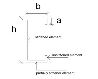
The distortional buckling is easy to occur for the cold-formed steel (CFS) lipped channel sections with holes. There is no design provision about effective width method (EWM) to predict the distortional buckling strength of CFS lipped channel sections with holes in China. His aim of this paper is to present an proposal of effective width method for the distortional buckling strength of CFS lipped channel sections with holes based on theoretical and numerical analysis on the partially stiffened element and CFS lipped channel section with holes. Firstly, the prediction methods for the distortional buckling stress and distortional buckling coefficients of CFS lipped channel sections with holes were developed based on the energy method and simplified rotation restrained stiffness. The accuracy of the proposed method for distortional buckling stress was verified by using the finite element method. Then the modified EWM was proposed to calculate the distortional buckling strength and the capacity of the interaction buckling of CFS lipped channel sections with holes based on the proposal of distortional buckling coefficient. Finally, comparisons on ultimate capacities of CFS lipped channel sections with holes of the calculated results by using the modified effective width method with 347 experimental results and 1598 numerical results indicated that the proposed EWM is reasonable and has a high accuracy and reliability for predicting the ultimate capacities of CFS lipped channel section with holes. Meanwhile, the predictions by the North America specification are slightly unconservative.
Citation: Xingyou Yao. EWM-based design method for distortional buckling of cold-formed thin-walled lipped channel sections with holes[J]. Mathematical Biosciences and Engineering, 2022, 19(1): 972-996. doi: 10.3934/mbe.2022045
The distortional buckling is easy to occur for the cold-formed steel (CFS) lipped channel sections with holes. There is no design provision about effective width method (EWM) to predict the distortional buckling strength of CFS lipped channel sections with holes in China. His aim of this paper is to present an proposal of effective width method for the distortional buckling strength of CFS lipped channel sections with holes based on theoretical and numerical analysis on the partially stiffened element and CFS lipped channel section with holes. Firstly, the prediction methods for the distortional buckling stress and distortional buckling coefficients of CFS lipped channel sections with holes were developed based on the energy method and simplified rotation restrained stiffness. The accuracy of the proposed method for distortional buckling stress was verified by using the finite element method. Then the modified EWM was proposed to calculate the distortional buckling strength and the capacity of the interaction buckling of CFS lipped channel sections with holes based on the proposal of distortional buckling coefficient. Finally, comparisons on ultimate capacities of CFS lipped channel sections with holes of the calculated results by using the modified effective width method with 347 experimental results and 1598 numerical results indicated that the proposed EWM is reasonable and has a high accuracy and reliability for predicting the ultimate capacities of CFS lipped channel section with holes. Meanwhile, the predictions by the North America specification are slightly unconservative.

| [1] |
S. C. W. Lau, G. J. Hancock, Distortional buckling formulas for channel columns, J. Struct. Eng., 113 (1987), 1063-1078. doi: 10.1061/(ASCE)0733-9445(1987)113:5(1063). doi: 10.1061/(ASCE)0733-9445(1987)113:5(1063)

|
| [2] | Y. B. Kwon, G. J. Hancock, Tests of cold-formed channels with local and distortional buckling. J. Struct. Eng., 118 (1992), 1786-1803. doi: 10.1061/(ASCE)0733-9445(1992)118:8(1786). |
| [3] |
G. J. Hancock, Design for distortional buckling of flexural members, Thin walled Struct., 27 (1997), 3-12. doi:10.1016/0263-8231(96)00020-1. doi: 10.1016/0263-8231(96)00020-1
|
| [4] |
B. W. Schafer, T. Pekoz, Laterally braced cold-formed steel flexural members with edge stiffened flanges, J. Struct. Eng., 125 (1999), 118-127. doi:10.1061/(ASCE)0733-9445(1999)125:2(118). doi: 10.1061/(ASCE)0733-9445(1999)125:2(118)
|
| [5] | B. W. Schafer, Local, distortional, and euler buckling of thin-walled columns, J. Struct. Eng., 128 (2002), 289-299. doi: 10.1061/(ASCE)0733-9445(2002)128:3(289). |
| [6] | X. Yao, Distortional buckling behavior and design method of cold-formed thin-walled steel sections, Tongji University, 2012. |
| [7] | X. Yao, Y. Li, Distortional buckling strength of cold-formed thin-walled steel members with lipped channel section, Eng. Mech., 31 (2014), 174-181. doi: 1000-4750(2014)09-0174-08. |
| [8] | R. A. Ortiz-Colberg, The load carrying capacity of perforated cold-formed steel columns, Cornell University, (1981), 152. |
| [9] | K. S. Sivakumaran. Load capacity of uniformly compressed cold-formed steel section with punched web, Can. J. Civ. Eng., 14 (1987), 550-558. doi: 10.1139/l87-080. |
| [10] | B. He, G. Zhao, Analysis on buckling behavior of cold-formed lipped channel with perforated web, J. Xi'an Inst. Met. Const. Eng., 21 (1989), 1-9. |
| [11] |
C. D. Moen, B. W. Schafer, Experiments on cold-formed steel columns with holes, Thin Walled Struct., 46 (2008), 1164-1182. doi: 10.1016/j.tws.2008.01.021. doi: 10.1016/j.tws.2008.01.021
|
| [12] | L. Xu, Y. Shi, S. Yang, Compressive strength of cold-formed steel c-shape columns with slotted holes, in Twenty-second international specialty conference on cold-formed steel structures: recent research and developments in cold-formed steel design and construction, (2014). Available from: https://scholarsmine.mst.edu/isccss/22iccfss/session02/4/. |
| [13] |
T. H. Miller, T. Pekoz, Unstiffened strip approach for perforated wall studs, J. Struct. Eng., 120 (1994), 410-421. doi: 10.1061/(ASCE)0733-9445(1994)120:2(410). doi: 10.1061/(ASCE)0733-9445(1994)120:2(410)
|
| [14] | N. Abdel-Rahman, Cold-formed steel compression members with perforations, PhD thesis, Mc Master University, Hamilton, Ontario, 1997. |
| [15] |
Y. Pu, M. H. R. Godley, R. G. Beale, H. Lau, Prediction of ultimate capacity of perforated lipped channels, J. Struct. Eng., 125 (1999), 510-514. doi: 10.1061/(ASCE)0733-9445(1999)125:5(510). doi: 10.1061/(ASCE)0733-9445(1999)125:5(510)
|
| [16] | B. Hu, Y. Liu, Ultimate capacities of cold-formed thin-walled channel columns with single hole under axial compression, J. Jiangsu Univ., 28 (2007), 258-261. doi: CNKI:SUN:JSLG.0.2007-03-018. |
| [17] |
Y. Guo, X. Yao, Distortional buckling behavior and design method of cold-formed steel lipped channel with rectangular holes under axial compression, Math. Bios. Eng., 18 (2021), 6239-6261. doi: 10.3934/mbe.2021312. doi: 10.3934/mbe.2021312
|
| [18] |
Y. Guo, X. Yao, Experimental study and effective width method for cold-formed steel lipped channel stud columns with holes, Adv. Civil Eng., 2021 (2021), 9949199. doi:10.1155/2021/9949199. doi: 10.1155/2021/9949199
|
| [19] |
X. Yao, Experimental investigation and load capacity of slender cold-formed lipped channel sections with holes in compression, Adv. Civil Eng., 2021 (2021), 6658099. doi:10.1155/2021/6658099. doi: 10.1155/2021/6658099
|
| [20] | J. Zhao, K. Sun, C. Yu, J. Wang. Tests and direct strength design on cold-formed steel channel beams with web holes. Eng. Struct., 184 (2019), 434-446. doi: 10.1016/j.engstruct.2019.01.062. |
| [21] |
C. D. Moen, A. Schudlich, A. Heyden, Experiments on cold-formed steel C-section joists with unstiffened web holes, J. Struct. Eng., 139 (2013), 695-704. doi: 10.1061/(ASCE)ST.1943-541X.0000652. doi: 10.1061/(ASCE)ST.1943-541X.0000652
|
| [22] | J. Zhou, S. Yu, Equiavalentcal calculation of buckling stress for cold-formed thin wall perforated channel columns, Steel. Const., 25 (2010), 27-31. |
| [23] |
C. D. Moen, B. W. Schafer, Elastic buckling of cold-formed steel columns and beams with holes, Eng. Struct., 31 (2009), 2812-2824. doi: 10.1016/j.engstruct.2009.07.007. doi: 10.1016/j.engstruct.2009.07.007
|
| [24] | X. Yao, Y. Guo, Y. Liu, J. Su, Y. Hu, Analysis on distortional buckling of cold-formed thin-walled steel lipped channel steel members with web openings under axial compression, Indust. Const., 50 (2020), 170-177. doi: 1000-4750(2014)09-0174-08. |
| [25] |
C. D. Moen, B. W. Schafer, Direct strength method for design of cold-formed steel columns with holes, J. Struct. Eng., 137 (2016), 559-570. doi: 10.1061/(ASCE)ST.1943-541X.0000310. doi: 10.1061/(ASCE)ST.1943-541X.0000310
|
| [26] |
Z. Yao, K. J. R. Rasmussen, Perforated cold-formed steel members in compression. Ⅱ: Design, J. Struct. Eng., 143 (2017), 04016227. doi:10.1061/(ASCE)ST.1943-541X.0001636. doi: 10.1061/(ASCE)ST.1943-541X.0001636
|
| [27] | American Iron and Steel Institute, North American specification for the design of cold-formed steel structural members, Canadian Standards Association, (2001). Available from: https://www.ce.jhu.edu/cfs/cfslibrary/AISI-S100-07%20Commentary.pdf. |
| [28] | Ministry of Housing and Urban-Rural Development of the People's Republic of China, Technical code for cold-formed thin-walled steel structures, Chinese Planning Press, (2002). |
| [29] |
A. Uzzaman, J. B. P. Lim, D. Nash, J. Rhodes, B. Young, Cold-formed steel sections with web openings subjected to web crippling under two-flange loading conditions-part I: tests and finite element analysis, Thin Walled Struct., 56 (2012), 38-48. doi: 10.1016/j.tws.2012.03.010. doi: 10.1016/j.tws.2012.03.010
|
| [30] |
A. Uzzaman, J. B. P. Lim, D. Nash, J. Rhodes, B. Young, Cold-formed steel sections with web openings subjected to web crippling under two-flange loading conditions-Part Ⅱ: parametric study and proposed design equations, Thin Walled Struct., 56 (2012), 79-87. doi: 10.1016/j.tws.2012.03.009. doi: 10.1016/j.tws.2012.03.009
|
| [31] |
Y. Lian, A. Uzzaman, J. B. Lim, G. Abdelal, D. Nash, B. Young, Effect of web holes on web crippling strength of cold-formed steel channel sections under end-one-flange loading condition-Part I: Tests and finite element analysis, Thin Walled Struct., 107 (2016), 443-452. doi: 10.1016/j.tws.2016.06.025. doi: 10.1016/j.tws.2016.06.025
|
| [32] |
Y. Lian, A. Uzzaman, J. B. Lim, G. Abdelal, D. Nash, B. Young, Effect of web holes on web crippling strength of cold-formed steel channel sections under end-one-flange loading condition-Part Ⅱ: Parametric study and proposed design equations, Thin Walled Struct., 107 (2016), 489-501. doi: 10.1016/j.tws.2016.06.026. doi: 10.1016/j.tws.2016.06.026
|
| [33] |
Y. Lian, A. Uzzaman, J. B. Lim, G. Abdelal, D. Nash, B. Young, Web crippling behaviour of cold-formed steel channel sections with web holes subjected to interior-one-flange loading condition-Part I: Experimental and numerical investigation, Thin Walled Struct., 111 (2017), 103-112. doi: 10.1016/j.tws.2016.10.024. doi: 10.1016/j.tws.2016.10.024
|
| [34] |
Y. Lian, A. Uzzaman, J. B. Lim, G. Abdelal, D. Nash, B. Young, Web crippling behaviour of cold-formed steel channel sections with web holes subjected to interior-one-flange loading condition-Part Ⅱ: parametric study and proposed design equations, Thin Walled Struct., 114 (2017), 92-106. doi: 10.1016/j.tws.2016.10.018. doi: 10.1016/j.tws.2016.10.018
|
| [35] |
C. H. Pham, Shear buckling of plates and thin-walled channel sections with holes, J. Constr. Steel Res., 128 (2017), 800-811. doi: 10.1016/j.jcsr.2016.10.013. doi: 10.1016/j.jcsr.2016.10.013
|
| [36] |
P. Keerthan, M. Mahendran, Improved shear design rules for lipped channel beams with web openings, J. Constr. Steel Res., 97 (2014), 127-142. doi: 10.1016/j.jcsr.2014.01.011. doi: 10.1016/j.jcsr.2014.01.011
|
| [37] |
B. Chen, K. Roy, A. Uzzaman, G. Raftery, J. B. P. Lim, Parametric study and simplified design equations for cold-formed steel channels with edge-stiffened holes under axial compression, J. Constr. Steel Res., 144 (2020), 106161. doi: 10.1016/j.jcsr.2020.106161. doi: 10.1016/j.jcsr.2020.106161
|
| [38] | B. Chen, K. Roy, A. Uzzaman, G. Raftery, J. B. P. Lim, Axial strength of back-to-back cold-formed steel channels with edge-stiffened holes, un-stiffened holes and plain webs, J. Constr. Steel Res., 174 (2020), 106313. doi: 10.1016/j.jcsr.2020.106313. |
| [39] |
A. Uzzaman, J. B. P. Lim, D. Nash, K. Roy, Web crippling behaviour of cold-formed steel channel sections with edge-stiffened and unstiffened circular holes under interior-two-flange loading condition, Thin Walled Struct., 154 (2020), 106813. doi: 10.1016/j.tws.2020.106813. doi: 10.1016/j.tws.2020.106813
|
| [40] | A. Uzzaman, J. B. P. Lim, D. Nash, K. Roy, Cold-formed steel channel sections under end-two-flange loading condition: Design for edge-stiffened holes, unstiffened holes and plain webs, Thin Walled Struct., 147 (2020), 106532. doi: 10.1016/j.tws.2019.106532. |
| [41] | B. Chen, K. Roy, A. Uzzaman, J. B. P. Lim, Moment capacity of cold-formed channel beams with edge-stiffened web holes, un-stiffened web holes and plain webs, Thin Walled Struct., 157 (2020), 107070. doi: 10.1016/j.tws.2020.107070. |
| [42] | ABAQUS, ABAQUS/Standard user's manual volumes I-Ⅲ and ABAQUS CAE manual, Dassault Systemes Simulia Corporation, (2014). Available from: https://xueshu.baidu.com/usercenter/paper/show?paperid=7918111e014ff6f8228180441bbaeead. |
| [43] | X. Yao, The buckling and interactive buckling behavior and design method of cold-formed steel lipped channel section with holes, Postdoctoral Report, Nanchang Institute of Technology, (2018). |


Figures(5) / Tables(11)

Xingyou Yao. EWM-based design method for distortional buckling of cold-formed thin-walled lipped channel sections with holes[J]. Mathematical Biosciences and Engineering, 2022, 19(1): 972-996. doi: 10.3934/mbe.2022045


 DownLoad: