Gastric cancer (GC) is the fifth most common malignancy and the fourth leading cause of cancer-related mortality worldwide. The identification of valuable predictive signatures to improve the prognosis of patients with GC is becoming a realistic prospect. DNA damage response-related long noncoding ribonucleic acids (drlncRNAs) play an important role in the development of cancers. However, their prognostic and therapeutic values remain sparse in gastric cancer (GC).
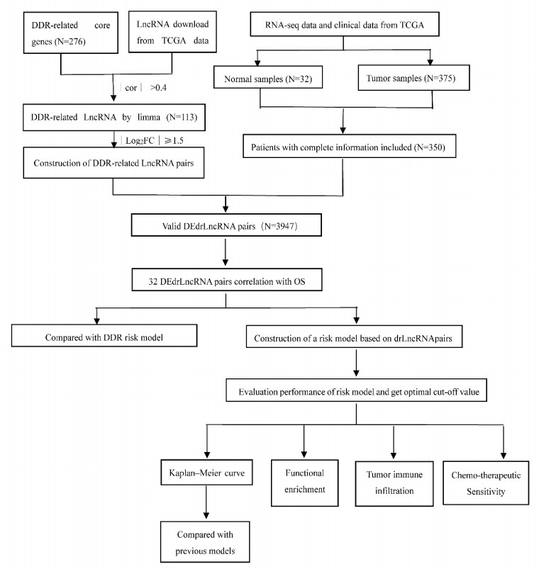
We obtained the transcriptome data and clinical information from The Cancer Genome Atlas Stomach Adenocarcinoma (TCGA-STAD) cohort. Co-expression network analyses were performed to discover functional modules using the igaph package. Subsequently, lncRNA pairs were identified by bioinformation analysis, and prognostic pairs were determined by univariate analysis, respectively. In addition, we utilized least absolute shrinkage and selection operator (LASSO) cox regression analysis to construct the risk model based on lncRNA pairs. Then, we distinguished between the high- or low- risk groups from patients with GC based on the optimal model. Finally, we reevaluated the association between risk score and overall survival, tumor immune microenvironment, specific tumor-infiltrating immune cells related biomarkers, and the sensitivity of chemotherapeutic agents.
32 drlncRNA pairs were obtained, and a 17-drlncRNA pairs signature was constructed to predict the overall survival of patients with GC. The ROC was 0.797, 0.812 and 0.821 at 1, 2, 3 years, respectively. After reclassifying these patients into different risk-groups, we could differentiate between them based on negative overall survival outcome, specialized tumor immune infiltration status, higher expressed immune cell related biomarkers, and a lower chemotherapeutics sensitivity. Compared with previous models, our model showed better performance with a higher ROC value.
The prognostic and therapeutic signature established by novel lncRNA pairs could provide promising prediction value, and guide individual treatment strategies in the future.
Citation: Yuan Yang, Lingshan Zhou, Xi Gou, Guozhi Wu, Ya Zheng, Min Liu, Zhaofeng Chen, Yuping Wang, Rui Ji, Qinghong Guo, Yongning Zhou. Comprehensive analysis to identify DNA damage response-related lncRNA pairs as a prognostic and therapeutic biomarker in gastric cancer[J]. Mathematical Biosciences and Engineering, 2022, 19(1): 595-611. doi: 10.3934/mbe.2022026
Gastric cancer (GC) is the fifth most common malignancy and the fourth leading cause of cancer-related mortality worldwide. The identification of valuable predictive signatures to improve the prognosis of patients with GC is becoming a realistic prospect. DNA damage response-related long noncoding ribonucleic acids (drlncRNAs) play an important role in the development of cancers. However, their prognostic and therapeutic values remain sparse in gastric cancer (GC).
We obtained the transcriptome data and clinical information from The Cancer Genome Atlas Stomach Adenocarcinoma (TCGA-STAD) cohort. Co-expression network analyses were performed to discover functional modules using the igaph package. Subsequently, lncRNA pairs were identified by bioinformation analysis, and prognostic pairs were determined by univariate analysis, respectively. In addition, we utilized least absolute shrinkage and selection operator (LASSO) cox regression analysis to construct the risk model based on lncRNA pairs. Then, we distinguished between the high- or low- risk groups from patients with GC based on the optimal model. Finally, we reevaluated the association between risk score and overall survival, tumor immune microenvironment, specific tumor-infiltrating immune cells related biomarkers, and the sensitivity of chemotherapeutic agents.
32 drlncRNA pairs were obtained, and a 17-drlncRNA pairs signature was constructed to predict the overall survival of patients with GC. The ROC was 0.797, 0.812 and 0.821 at 1, 2, 3 years, respectively. After reclassifying these patients into different risk-groups, we could differentiate between them based on negative overall survival outcome, specialized tumor immune infiltration status, higher expressed immune cell related biomarkers, and a lower chemotherapeutics sensitivity. Compared with previous models, our model showed better performance with a higher ROC value.
The prognostic and therapeutic signature established by novel lncRNA pairs could provide promising prediction value, and guide individual treatment strategies in the future.

| [1] |
H. Sung, J. Ferlay, R. L. Siegel, M. Laversanne, I. Soerjomataram, A. Jemal, et al., Global cancer statistics 2020: GLOBOCAN estimates of incidence and mortality worldwide for 36 cancers in 185 countries, CA. Cancer J. Clin., 3 (2021), 209–249. doi: 10.3322/caac.21660. doi: 10.3322/caac.21660

|
| [2] |
P. H. Viale, The american cancer society's facts & figures: 2020 edition, J. Adv. Pract. Oncol., 11 (2020), 135–136. doi: 10.6004/jadpro.2020.11.2.1. doi: 10.6004/jadpro.2020.11.2.1
|
| [3] |
A. D. Wagner, N. L. Syn, M. Moehler, W. Grothe, W. P. Yong, B. Tai, et al., Chemotherapy for advanced gastric cancer, Cochrane Database Syst. Rev., 8 (2017), CD004064. doi: 10.1002/14651858.CD004064.pub4. doi: 10.1002/14651858.CD004064.pub4
|
| [4] |
J. J. G. Marin, L. Perez-Silva, R. I. R. Macias, M. Asensio, A. Peleteiro-Vigil, A. Sanchez-Martin, et al., Molecular bases of mechanisms accounting for drug resistance in gastric adenocarcinoma, Cancers (Basel), 12 (2020), 2116. doi: 10.3390/cancers12082116. doi: 10.3390/cancers12082116
|
| [5] |
L. H. Pearl, A. C. Schierz, S. E. Ward, B. Al-Lazikani, F. M. G. Pearl, Therapeutic opportunities within the DNA damage response, Nat. Rev. Cancer, 15 (2015), 166–180. doi: 10.1038/nrc3891. doi: 10.1038/nrc3891
|
| [6] |
Cancer Genome Atlas Research Network, Comprehensive molecular characterization of gastric adenocarcinoma, Nature, 513 (2014), 202–209. doi: 10.1038/nature13480. doi: 10.1038/nature13480
|
| [7] |
V. Krishnan, I. Orcid, D. X. E. Lim, S. Srivastava, J. Matsuo, K. K. Huang, et al., DNA damage signalling as an anti-cancer barrier in gastric intestinal metaplasia, Gut, 69 (2020), 1738–1749. doi: 10.1136/gutjnl-2019-319002. doi: 10.1136/gutjnl-2019-319002
|
| [8] |
M. J. O' Conno, Targeting the DNA damage response in cancer, Mol. Cell, 60 (2015), 547–560. doi: 10.1016/j.molcel.2015.10.040. doi: 10.1016/j.molcel.2015.10.040
|
| [9] |
H. E. Lee, N. Han, M. A. Kim, H. S. Lee, H. Yang, B. L. Lee, et al., DNA damage response-related proteins in gastric cancer: ATM, Chk2 and p53 expression, Pathobiology, 81 (2014), 25–35. doi: 10.1159/000351072. doi: 10.1159/000351072
|
| [10] |
Y. Fang, M. J. Fullwood, Roles, functions, and mechanisms of long non-coding RNAs in cancer, Genomics Proteomics bioinf., 14 (2016), 42–54. doi: 10.1016/j.gpb.2015.09.006. doi: 10.1016/j.gpb.2015.09.006
|
| [11] |
S. Xie, Y. Chang, H. Jin, F. Yang, Y. Xu, X. Yan, et al., Non-coding RNAs in gastric cancer, Cancer Lett., 493 (2020), 55–70. doi: 10.1016/j.canlet.2020.06.022. doi: 10.1016/j.canlet.2020.06.022
|
| [12] |
F. Michelini, S. Pitchiaya, I. Orcid, S. Sharma, U. Gioia, F. Pessina, et al., Damage-induced lncRNAs control the DNA damage response through interaction with DDRNAs at individual double-strand breaks, Nat. Cell Biol., 19 (2017), 1400–1411. doi: 10.1038/ncb3643. doi: 10.1038/ncb3643
|
| [13] |
F. Pessina, F. Giavazzi, I. Orcid, U. Gioia, V. Vitelli, A. Galbiati, et al., Functional transcription promoters at DNA double-strand breaks mediate RNA-driven phase separation of damage-response factors, Nat. Cell Biol., 21 (2019), 1286–1299. doi: 10.1038/s41556-019-0392-4. doi: 10.1038/s41556-019-0392-4
|
| [14] |
H. Zhang, Y. Hua, Z. Jiang, J. Yue, M. Shi, X. Zhen, et al., Cancer-associated fibroblast-promoted LncRNA DNM3OS confers radioresistance in esophageal squamous cell carcinoma, Clin. Cancer Res., 25 (2019), 1989–2000. doi: 10.1158/1078-0432.CCR-18-0773. doi: 10.1158/1078-0432.CCR-18-0773
|
| [15] |
T. A. Knijnenburg, L. Wang, M. T. Zimmermann, N. Chambwe, G. F. Ga, A. D. Cherniack, et al., Genomic and molecular landscape of DNA damage repair deficiency across The Cancer Genome Atlas, Cell Rep., 1 (2018), 239–254. doi: 10.1016/j.celrep.2018.03.076. doi: 10.1016/j.celrep.2018.03.076
|
| [16] |
W. Hong, L. Liang, Y. Gu, Z. Qi, H. Qiu, X. Yang, et al., Immune-related lncRNA to construct novel signature and predict the immune landscape, Mol. Ther. Nucleic Acids, 22 (2020), 937–947. doi: 10.1016/j.omtn.2020.10.002. doi: 10.1016/j.omtn.2020.10.002
|
| [17] |
C. Nastasi, L. Mannarino, M. D'Incalci, DNA damage response and immune defense, Int. J. Mol. Sci., 21 (2020), 7504. doi: 10.3390/ijms21207504. doi: 10.3390/ijms21207504
|
| [18] |
X. Zhang, Y. Peng, Y. Yuan, Y. Gao, F. Hu, J. Wang, et al., Histone methyltransferase SET8 is regulated by miR-192/215 and induces oncogene-induced senescence via p53-dependent DNA damage in human gastric carcinoma cells, Cell Death Dis., 11 (2020), 937. doi: 10.1038/s41419-020-03130-4. doi: 10.1038/s41419-020-03130-4
|
| [19] |
C. Xie, N. Li, H. Wang, C. He, Y. Hu, C. Peng, et al., Inhibition of autophagy aggravates DNA damage response and gastric tumorigenesis via Rad51 ubiquitination in response to H. pylori infection, Gut Microbes, 11 (2020), 1567–1589. doi: 10.1080/19490976.2020.1774311. doi: 10.1080/19490976.2020.1774311
|
| [20] |
F. S. Manoel-Caetano, A. F. T. Rossi, C. G. Morais, F. E. Severino, A. E. Silva, Upregulation of the APE1 and H2AX genes and miRNAs involved in DNA damage response, Genes Dis., 6 (2019), 176–184. doi: 10.1016/j.gendis.2019.03.007. doi: 10.1016/j.gendis.2019.03.007
|
| [21] |
H. Cai, C. Jing, X. Chang, D. Ding, T. Han, J. Yang, et al., Mutational landscape of gastric cancer and clinical application of genomic profiling based on target next-generation sequencing, J. Transl. Med., 17 (2019), 189. doi: 10.1186/s12967-019-1941-0. doi: 10.1186/s12967-019-1941-0
|
| [22] |
S. Ghafouri-Fard, M. Taheri, Long non-coding RNA signature in gastric cancer, Exp. Mol. Pathol., 113 (2020), 104365. doi: 10.1016/j.yexmp.2019.104365. doi: 10.1016/j.yexmp.2019.104365
|
| [23] |
H. Arai, R. Wada, K. Ishino, M. Kudo, E. Uchida, Z. Naito, Expression of DNA damage response proteins in gastric cancer: Comprehensive protein profiling and histological analysis, Int. J. Oncol., 52 (2018), 978–988. doi: 10.3892/ijo.2018.4238. doi: 10.3892/ijo.2018.4238
|
| [24] |
Y. Wu, J. Deng, S. Lai, Y. You, J. Wu, A risk score model with five long non-coding RNAs for predicting prognosis in gastric cancer: an integrated analysis combining TCGA and GEO datasets, PeerJ, 9 (2021), e10556. doi: 10.7717/peerj.10556. doi: 10.7717/peerj.10556
|
| [25] |
Z. H. Ma, Y. Shuai, X. Y. Gao, Y. Yan, K. M. Wang, X. Z. Wen, et al., BTEB2-Activated lncRNA TSPEAR-AS2 drives GC progression through suppressing GJA1 and upregulating CLDN4 expression, Mol. Ther. Nucleic Acids, 22 (2020), 1129–1141. doi: 10.1016/j.omtn.2020.10.022. doi: 10.1016/j.omtn.2020.10.022
|
| [26] |
L. Yu, W. Luan, Z. Feng, J. Jia, Z. Wu, M. Wang, et al., Long non-coding RNA HAND2-AS1 inhibits gastric cancer progression by suppressing TCEAL7 expression via targeting miR-769-5p, Dig. Liver Dis., 2 (2021), 238–244. doi: 10.1016/j.dld.2020.08.045. doi: 10.1016/j.dld.2020.08.045
|
| [27] |
T. Reisländer, F. J. Groelly, M. Tarsounas, DNA damage and cancer immunotherapy: a STING in the tale, Mol. Cell, 1 (2020), 21–28. doi: 10.1016/j.molcel.2020.07.026. doi: 10.1016/j.molcel.2020.07.026
|
| [28] |
B. S. Parker, J. Rautela, P. J. Hertzog, Antitumour actions of interferons: implications for cancer therapy, Nat. Rev. Cancer, 3 (2016), 131–144. doi: 10.1038/nrc.2016.14. doi: 10.1038/nrc.2016.14
|
| [29] |
T. Sen, B. L. Rodriguez, L. Chen, C. M. D Corte, N. Morikawa, J. Fujimoto, et al., Targeting DNA damage response promotes antitumor immunity through STING-mediated T-cell activation in small cell lung cancer, Cancer Discov., 5 (2019), 646–661. doi: 10.1158/2159-8290.CD-18-1020. doi: 10.1158/2159-8290.CD-18-1020
|
| [30] |
H. Zhang, T. Deng, R. Liu, T. Ning, H. Yang, D. Liu, et al., CAF secreted miR-522 suppresses ferroptosis and promotes acquired chemo-resistance in gastric cancer, Mol. Cancer, 1 (2020), 43. doi: 10.1186/s12943-020-01168-8. doi: 10.1186/s12943-020-01168-8
|
| [31] |
X. Meng, C. Duan, H. Pang, Q. Chen, B. Han, C. Zha, et al., DNA damage repair alterations modulate M2 polarization of microglia to remodel the tumor microenvironment via the p53-mediated MDK expression in glioma, EBioMedicine, 41 (2019), 185–199. doi: 10.1016/j.ebiom.2019.01.067. doi: 10.1016/j.ebiom.2019.01.067
|
| [32] |
A. Sistigu, T. Yamazaki, E. Vacchelli, K. Chaba, D.P. Enot, J. Adam, et al., Cancer cell-autonomous contribution of type Ⅰ interferon signaling to the efficacy of chemotherapy, Nat. Med., 11 (2014), 1301–1309. doi: 10.1038/nm.3708. doi: 10.1038/nm.3708
|
 mbe-19-01-026-Supplementary.zip mbe-19-01-026-Supplementary.zip |
 |


Figures(8)

Yuan Yang, Lingshan Zhou, Xi Gou, Guozhi Wu, Ya Zheng, Min Liu, Zhaofeng Chen, Yuping Wang, Rui Ji, Qinghong Guo, Yongning Zhou. Comprehensive analysis to identify DNA damage response-related lncRNA pairs as a prognostic and therapeutic biomarker in gastric cancer[J]. Mathematical Biosciences and Engineering, 2022, 19(1): 595-611. doi: 10.3934/mbe.2022026


 DownLoad: