Numerical assessment of directional energy performance for 3D printed midsole structures

Ankhy Sultana; Tsz-Ho Kwok; Hoi Dick Ng; Ankhy Sultana; Tsz-Ho Kwok; Hoi Dick Ng

doi:10.3934/mbe.2021224

Mathematical Biosciences and Engineering

2021, Volume 18, Issue 4: 4429-4449. doi: 10.3934/mbe.2021224

Previous Article Next Article

Research article Special Issues

Numerical assessment of directional energy performance for 3D printed midsole structures

Department of Mechanical, Industrial and Aerospace Engineering, Concordia University, 1455 de Maisonneuve Blvd. W., Montreal, QC H3G 1M8, Canada

Received: 01 March 2021 Accepted: 18 May 2021 Published: 24 May 2021

Energy can be represented in the form of deformation obtained by the applied force. Energy transfer is defined in physics as the energy is moved from one place to another. To make the energy transfer functional, energy should be moved into the right direction. If it is possible to make a better use of the energy in the right direction, the energy efficiency of the structure can be enhanced. This idea leads to the concept of directional energy transfer (DET), which refers to transferring energy from one direction to a specific direction. With the recent development of additive manufacturing and topology optimization, complex structures can be applied to various applications to enhance performances, like a wheel and shoe midsole. While many works are related to structural strength, there is limited research in optimization for energy performance. In this study, a theoretical approach is proposed to measure the directional energy performance of a structure, which can be used to measure the net energy in an intended direction. The purpose is to understand the energy behavior of a structure and to measure if a structure is able to increase energy in the desired direction.
- directional energy transfer,
- structure,
- lattice,
- simulation,
- modeling,
- shoe midsole
Citation: Ankhy Sultana, Tsz-Ho Kwok, Hoi Dick Ng. Numerical assessment of directional energy performance for 3D printed midsole structures[J]. Mathematical Biosciences and Engineering, 2021, 18(4): 4429-4449. doi: 10.3934/mbe.2021224

Related Papers:

Abstract

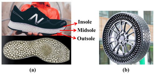
Energy can be represented in the form of deformation obtained by the applied force. Energy transfer is defined in physics as the energy is moved from one place to another. To make the energy transfer functional, energy should be moved into the right direction. If it is possible to make a better use of the energy in the right direction, the energy efficiency of the structure can be enhanced. This idea leads to the concept of directional energy transfer (DET), which refers to transferring energy from one direction to a specific direction. With the recent development of additive manufacturing and topology optimization, complex structures can be applied to various applications to enhance performances, like a wheel and shoe midsole. While many works are related to structural strength, there is limited research in optimization for energy performance. In this study, a theoretical approach is proposed to measure the directional energy performance of a structure, which can be used to measure the net energy in an intended direction. The purpose is to understand the energy behavior of a structure and to measure if a structure is able to increase energy in the desired direction.

References

[1]	F. K. Fuss, Function or fashion? Design of sports shoes and directional energy return: Introducing a new concept of directional energy transfer, in The Impact of Technology on Sport III, (2009), 167–171.
[2]	S. Guide, Anatomy of the shoe. Available from: https://www.shoeguide.org/shoe_anatomy/.
[3]	D. T. P. Fong, Y. Hong, J. X. Li, Cushioning and lateral stability functions of cloth sport shoes, Sports Biomech., 6 (2007), 407–417. doi: 10.1080/14763140701491476
[4]	H. Elftman, The force exerted by the ground in walking, Arbeitsphysiologie, 10 (1939), 485–491.
[5]	D. J. Stefanyshyn, B. M. Nigg, Energy and performance aspects in sport surfaces, Sports Biomech., (2003), 31–46.
[6]	G. Baroud, B. M. Nigg, D. Stefanyshyn, Energy storage and return in sport surfaces, Sports Eng., 2 (1999), 173–180. doi: 10.1046/j.1460-2687.1999.00031.x
[7]	T. A. McMahon, P. R. Green, Fast running tracks, Sci. Am., 239 (1978), 148–163.
[8]	T. A. McMahon, P. R. Greene, The influence of track compliance on running, J. Biomech., 12 (1979), 893–904. doi: 10.1016/0021-9290(79)90057-5
[9]	E. C. Frederick, E. T. Howley, S. K. Powers, Lower oxygen demands of running in soft-soled shoes, Res. Q. Exercise Sport, 57 (1986), 174–177. doi: 10.1080/02701367.1986.10762196
[10]	C. E. Rothschild, Primitive running: A survey analysis of runners' interest, participation, and implementation, J. Strength Cond. Res., 26 (2012), 2021–2026. doi: 10.1519/JSC.0b013e31823a3c54
[11]	E. M. Hennig, Eighteen years of running shoe testing in germany – a series of biomechanical studies, Footwear Sci., 3 (2011), 71–81. doi: 10.1080/19424280.2011.616536
[12]	J. T. Fuller, C. R. Bellenger, D. Thewlis, M. D. Tsiros, J. D. Buckley, The effect of footwear on running performance and running economy in distance runners, Sports Med., 45 (2015), 411–422. doi: 10.1007/s40279-014-0283-6
[13]	N. Guo, M. C. Leu, Additive manufacturing: technology, applications and research needs, Front. Mechan. Eng., 8 (2013), 215–243. doi: 10.1007/s11465-013-0248-8
[14]	Y. S. Leung, T. H. Kwok, X. Li, Y. Yang, C. C. L. Wang, Y. Chen, Challenges and status on design and computation for emerging additive manufacturing technologies, ASME. J. Comput. Inf. Sci. Eng., 19 (2019), 021013. doi: 10.1115/1.4041913
[15]	W. Tao, M. C. Leu, Design of lattice structure for additive manufacturing, in 2016 International Symposium on Flexible Automation (ISFA), (2016), 325–332.
[16]	M. Mazur, M. Leary, S. Sun, M. Vcelka, D. Shidid, M. Brandt, Deformation and failure behaviour of Ti-6Al-4V lattice structures manufactured by selective laser melting (SLM), Int. J. Adv. Manuf. Technol., 84 (2016), 1391–1411.
[17]	J. Wallach, L. Gibson, Mechanical behavior of a three-dimensional truss material, Int. J. Solids Struct., 38 (2001), 7181–7196. doi: 10.1016/S0020-7683(00)00400-5
[18]	Z. Xiao, Y. Yang, R. Xiao, Y. Bai, C. Song, D. Wang, Evaluation of topology-optimized lattice structures manufactured via selective laser melting, Mater. Des., 143 (2018), 27–37. doi: 10.1016/j.matdes.2018.01.023
[19]	J. Martínez, S. Hornus, H. Song, S. Lefebvre, Polyhedral voronoi diagrams for additive manufacturing, ACM Trans. Graph., 37 (2018), 1–15.
[20]	H. Xu, Y. Li, Y. Chen, J. Barbič, Interactive material design using model reduction, ACM Trans. Graph., 34 (2015), 1–14.
[21]	T. Shepherd, K. Winwood, P. Venkatraman, A. Alderson, T. Allen, Validation of a finite element modeling process for auxetic structures under impact, Phys. Status Solidi B, 257 (2020), 190–197.
[22]	B. Nigg, B. Segesser, Biomechanical and orthopedic concepts in sport shoe construction, Med. Sci. Sports Exercise, 24, (1992), 595–602.
[23]	C. Reinschmidt, B. M. Nigg, Current issues in the design of running and court shoes, Sportverletzung Sportschaden, 14 (2000), 71–81.
[24]	B. Braunstein, A. Arampatzis, P. Eysel, G.-P. Brüggemann, Footwear affects the gearing at the ankle and knee joints during running, J. Biomech., 43 (2010), 2120–2125. doi: 10.1016/j.jbiomech.2010.04.001
[25]	B. Nigg, M. Morlock, The influence of lateral heel flare of running shoes on pronation and impact forces, Med. Sci. Sports Exercise, 19 (1997), 294–302.
[26]	R. W. Bohannon, A. W. Andrews, Normal walking speed: a descriptive meta-analysis, Physiotherapy, 97 (2011), 182–189. doi: 10.1016/j.physio.2010.12.004
[27]	J. Bonacci, P. U. Saunders, A. Hicks, T. Rantalainen, B. G. T. Vicenzino, W. Spratford, Running in a minimalist and lightweight shoe is not the same as running barefoot: a biomechanical study, Br. J. Sports Med., 47 (2013), 387–392. doi: 10.1136/bjsports-2012-091837
[28]	S. Willwacher, M. Konig, W. Potthast, G.-P. Bruggemann, Does specific footwear facilitate energy storage and return at the metatarsophalangeal joint in running?, J. Appl. Biomech., 29 (2013), 583–592. doi: 10.1123/jab.29.5.583
[29]	M. J. Dickson, F. K. Fuss, Optimization of directional energy transfer in adidas bounce tubes, Proceed. Eng., 2 (2010), 2795–2800. doi: 10.1016/j.proeng.2010.04.068
[30]	M. J. Dickson, F. K. Fuss, Effect of acceleration on optimization of adidas bounce shoes, Proced. Eng., 13 (2011), 107–112. doi: 10.1016/j.proeng.2011.05.059
[31]	M. J. Dickson, Optimization of Directional Energy Transfer in Running Shoes. PhD Thesis, RMIT University, Melbourne, VC, September 2014.
[32]	M. Müller, M. Gross, Interactive virtual materials, in Proceedings of Graphics Interface 2004, (2004), 239–246.

Reader Comments

Your name:*

Email:*
© 2021 the Author(s), licensee AIMS Press. This is an open access article distributed under the terms of the Creative Commons Attribution License (http://creativecommons.org/licenses/by/4.0)