Generative adversarial network based data augmentation to improve cervical cell classification model

Suxiang Yu; Shuai Zhang; Bin Wang; Hua Dun; Long Xu; Xin Huang; Ermin Shi; Xinxing Feng; Suxiang Yu; Shuai Zhang; Bin Wang; Hua Dun; Long Xu; Xin Huang; Ermin Shi; Xinxing Feng

doi:10.3934/mbe.2021090

Mathematical Biosciences and Engineering

2021, Volume 18, Issue 2: 1740-1752. doi: 10.3934/mbe.2021090

Previous Article Next Article

Research article Special Issues

Generative adversarial network based data augmentation to improve cervical cell classification model

1.
Department of Pathology, The Fourth Central Hospital of Baoding City, Baoding 072350, China
2.
Department of Computer Science, The University of Manchester, Manchester M13 9PL, UK
3.
Solar Activity Prediction Center, National Astronomical Observatories, Chinese Academy of Sciences, Beijing 100012, China
4.
Department of Information Technology, The Fourth Central Hospital of Baoding City, Baoding 072350, China
5.
Endocrinology and Cardiovascular Disease Centre, Fuwai Hospital, National Center for Cardiovascular Diseases, Chinese Academy of Medical Sciences and Peking Union Medical College, Beijing 100037, China
^† These two authors contributed equally.

Received: 26 October 2020 Accepted: 20 January 2021 Published: 08 February 2021

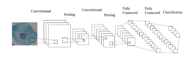
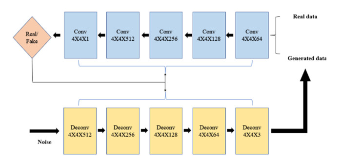
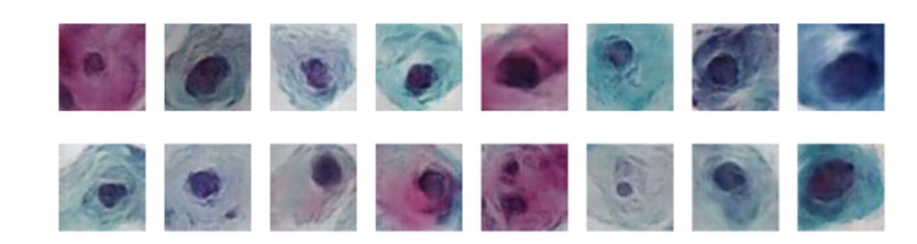
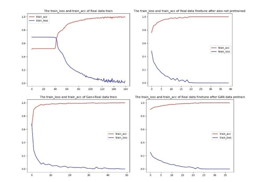
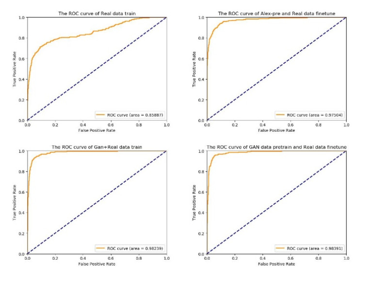
The survival rate of cervical cancer can be improved by the early screening. However, the screening is a heavy task for pathologists. Thus, automatic cervical cell classification model is proposed to assist pathologists in screening. In cervical cell classification, the number of abnormal cells is small, meanwhile, the ratio between the number of abnormal cells and the number of normal cells is small too. In order to deal with the small sample and class imbalance problem, a generative adversarial network (GAN) trained by images of abnormal cells is proposed to obtain the generated images of abnormal cells. Using both generated images and real images, a convolutional neural network (CNN) is trained. We design four experiments, including 1) training the CNN by under-sampled images of normal cells and the real images of abnormal cells, 2) pre-training the CNN by other dataset and fine-tuning it by real images of cells, 3) training the CNN by generated images of abnormal cells and the real images, 4) pre-training the CNN by generated images of abnormal cells and fine-tuning it by real images of cells. Comparing these experimental results, we find that 1) GAN generated images of abnormal cells can effectively solve the problem of small sample and class imbalance in cervical cell classification; 2) CNN model pre-trained by generated images and fine-tuned by real images achieves the best performance whose AUC value is 0.984.
- cervical cell classification,
- data augmentation,
- generative adversarial network (GAN),
- deep learning
Citation: Suxiang Yu, Shuai Zhang, Bin Wang, Hua Dun, Long Xu, Xin Huang, Ermin Shi, Xinxing Feng. Generative adversarial network based data augmentation to improve cervical cell classification model[J]. Mathematical Biosciences and Engineering, 2021, 18(2): 1740-1752. doi: 10.3934/mbe.2021090

Related Papers:

Abstract

The survival rate of cervical cancer can be improved by the early screening. However, the screening is a heavy task for pathologists. Thus, automatic cervical cell classification model is proposed to assist pathologists in screening. In cervical cell classification, the number of abnormal cells is small, meanwhile, the ratio between the number of abnormal cells and the number of normal cells is small too. In order to deal with the small sample and class imbalance problem, a generative adversarial network (GAN) trained by images of abnormal cells is proposed to obtain the generated images of abnormal cells. Using both generated images and real images, a convolutional neural network (CNN) is trained. We design four experiments, including 1) training the CNN by under-sampled images of normal cells and the real images of abnormal cells, 2) pre-training the CNN by other dataset and fine-tuning it by real images of cells, 3) training the CNN by generated images of abnormal cells and the real images, 4) pre-training the CNN by generated images of abnormal cells and fine-tuning it by real images of cells. Comparing these experimental results, we find that 1) GAN generated images of abnormal cells can effectively solve the problem of small sample and class imbalance in cervical cell classification; 2) CNN model pre-trained by generated images and fine-tuned by real images achieves the best performance whose AUC value is 0.984.

References

[1]	L. Torre, F. Bray, R. L. Siegel, J. Ferlay, J. Lortet-Tieulent, A. Jemal, Global cancer statistics, 2012, CA Cancer J. Clin., 65 (2015), 87–108.
[2]	S. Chen, D. Gao, L. Wang, Y. Zhang, Cervical Cancer Single Cell Image Data Augmentation Using Residual Condition Generative Adversarial Networks, 2020 3rd International Conference on Artificial Intelligence and Big Data (ICAIBD), 2020.
[3]	D. Xue, X. Zhou, C. Li, Y. Yao, M. M. Rahaman, J. Zhang. et al., An Application of Transfer Learning and Ensemble Learning Techniques for Cervical Histopathology Image Classification, IEEE Access, 8 (2020), 104603–104618. doi: 10.1109/ACCESS.2020.2999816
[4]	N. Sompawong, J. Mopan, P. Pooprasert, W. Himakhun, K. Suwannarurk, J. Ngamvirojcharoen, et al., Automated pap smear cervical cancer screening using deep learning, 41st Annual International Conference of the IEEE Engineering in Medicine and Biology Society (EMBC), 2019.
[5]	M. Wu, C. Yan, H. Liu, Q. Liu, Y. Yin, Automatic classification of cervical cancer from cytological images by using convolutional neural network, Biosci. Rep., 6 (2018), 38.
[6]	O. E. Aina, S. A. Adeshina, A. M. Aibinu, Classification of Cervix types using Convolution Neural Network (CNN), 15th International Conference on Electronics, Computer and Computation (ICECCO), 2019.
[7]	P. B. Shanthi, F. Faruqi, K. S. Hareesha, K. Ranjini, Deep convolution neural network for malignancy detection and classification in microscopic uterine cervix cell images, Asian Pac. J. Cancer Prev., 20 (2019), 3447–3456. doi: 10.31557/APJCP.2019.20.11.3447
[8]	H. Lin, Y. Hu, S. Chen, J. Yao, L. Zhang, Fine-grained classification of cervical cells using morphological and appearance based convolutional neural networks, IEEE Access, 7 (2019), 71541–71549. doi: 10.1109/ACCESS.2019.2919390
[9]	J. Payette, J. Rachleff, C. V. Graaf, Intel and MobileODT Cervical Cancer Screening Kaggle Competition: cervix type classification using Deep Learning and image classification, 2017. Available from: http://cs231n.stanford.edu/reports/2017/pdfs/923.pdf.
[10]	M. Kwon, M. Kuko, M. Pourhomayoun, V. Martin, T. H. Kim, S. E. Martin, Multi-label classification of single and clustered cervical cells using deep convolutional networks, California State University, Los Angeles, 2018.
[11]	Kurnianingsih, K. H. S. Allehaibi, L. E. Nugroho, Widyawan, L. Lazuardi, A. S. Prabuwono, et al., Segmentation and classification of cervical cells using deep learning, IEEE Access, 7 (2019), 116925–116941. doi: 10.1109/ACCESS.2019.2936017
[12]	Y. Xue, Q. Zhou, J. Ye, L. R. Long, S. Antani, C. Cornwell, et al., Synthetic augmentation and feature-based filtering for improved cervical histopathology image classification, International conference on medical image computing and computer-assisted intervention. Springer, Cham, 2019.
[13]	W. William, A. Ware, A. H. Basaza-Ejiri, J. Obungoloch, A review of image analysis and machine learning techniques for automated cervical cancer screening from pap-smear images, Comput. Methods Programs Biomed., 164 (2018), 15–22.
[14]	N. V. Chawla, Data mining for imbalanced datasets: An overview, in Data Mining and Knowledge Discovery Handbook, Springer, Boston, MA, 2009,875–886.
[15]	X. Y. Liu, J. Wu, Z. H. Zhou, Exploratory undersampling for class-imbalance learning, IEEE Trans. Syst. Man Cybern. Part B, 39 (2009), 539–550. doi: 10.1109/TSMCB.2008.2007853
[16]	I. Mani, I. Zhang, kNN approach to unbalanced data distributions: a case study involving information extraction, Proceedings of workshop on learning from imbalanced datasets, 2003.
[17]	I. Tomek, Two Modifications of CNN, IEEE Trans. Syst. Man Cybern., 11 (1976), 769–772.
[18]	I. Tomek, An Experiment with the Edited Nearest-Neighbor Rule, IEEE Trans. Syst. Man Cybern., 6 (1976), 448–452.
[19]	C. X. Ling, C. Li, Data mining for direct marketing: Problems and solutions, Plenary Presentation, 98 (1998), 73–79.
[20]	N. V. Chawla, K. W. Bowyer, L. O. Hall, W. P. Kegelmeyer, SMOTE: Synthetic Minority Over-sampling Technique, J. Artif. Intell. Res., 16 (2002), 321–357. doi: 10.1613/jair.953
[21]	H. Han, W. Y. Wang, B. H. Mao, Borderline-SMOTE: a new over-sampling method in imbalanced data sets learning, International conference on intelligent computing. Springer, Berlin, Heidelberg, 2005.
[22]	X. Li, L. Wang, E. Sung, AdaBoost with SVM-based component classifiers, Eng. Appl. Artif. Intell., 21 (2008), 785–795. doi: 10.1016/j.engappai.2007.07.001
[23]	A. Liu, J. Ghosh, C. E. Martin, Generative Oversampling for Mining Imbalanced Datasets, DMIN, 2007, 66–72.
[24]	B. Chen, Y. D. Su, S. Huang, Classification of imbalance data based on KM-SMOTE algorithm and random forest, Comput. Technol. Dev., 5 (2015), 17–21.
[25]	G. E. Batista, R. C. Prati, M. C. Monard, A study of the behavior of several methods for balancing machine learning training data, ACM SIGKDD Explor. Newsl., 6 (2004), 20–29. doi: 10.1145/1007730.1007735
[26]	W. Fan, S. J. Stolfo, J. Zhang, P. K. Chan, AdaCost: misclassification cost-sensitive boosting, ICML, 1999.
[27]	P. Chen, S. Liu, H. Zhao, J. Jia, Grid Mask data augmentation, preprint, arXiv: 2001.04086.
[28]	S. Yun, D. Han, S. J. Oh, S. Chun, J. Choe, Y. Yoo, Cutmix: Regularization strategy to train strong classifiers with localizable features, Proceedings of the IEEE International Conference on Computer Vision, 2019.
[29]	H. Zhang, M. Cisse, Y. N. Dauphin, D. Lopez-Paz, Mixup: Beyond empirical risk minimization, preprint, arXiv: 1710.09412.
[30]	H. Inoue, Data augmentation by pairing samples for images classification, preprint, arXiv: 1801.02929.
[31]	J. Lemley, S. Bazrafkan, P. Corcoran, Smart augmentation learning an optimal data augmentation strategy, IEEE Access, 5 (2017), 5858–5869. doi: 10.1109/ACCESS.2017.2696121
[32]	I. Goodfellow, J. Pouget-Abadie, M. Mirza, B. Xu, D. Warde-Farley, S. Ozair, et al., Generative adversarial nets, Advances in neural information processing systems, 2014.
[33]	B. Li, F. Wu, S. N. Lim, S. Belongie, K. Q. Weinberger, On Feature Normalization and Data Augmentation, preprint, arXiv: 2002.11102.
[34]	E. D. Cubuk, B. Zoph, D. Mane, V. Vasudevan, Q. V. Le, Autoaugment: Learning augmentation strategies from data, Proceedings of the IEEE Conference on Computer Vision and Pattern Recognition, 2019.
[35]	A. Krizhevsky, I. Sutskever, G. E. Hinton, Imagenet classification with deep convolutional neural networks, Adv. Neural Inf. Proc. Syst., 25 (2012), 1097–1105.
[36]	M. Frid-Adar, I. Diamant, E. Klang, M. Amitai, J. Goldberger, H. Greenspan, GAN-based Synthetic Medical Image Augmentation for increased CNN Performance in Liver Lesion Classification, Neurocomputing, 321 (2018), 321–331. doi: 10.1016/j.neucom.2018.09.013
[37]	M. Frid-Adar, E. Klang, M. Amitai, J. Goldberger, H. Greenspan, Synthetic data augmentation using GAN for improved liver lesion classification, Proceedings of the 2018 IEEE 15th International Symposium on Biomedical Imaging, Washington, DC, 2018.
[38]	Y. Onishi, A. Teramoto, M. Tsujimoto, T. Tsukamoto, K. Saito, H. Toyama, et al., Automated Pulmonary Nodule Classification in Computed Tomography Images Using a Deep Convolutional Neural Network Trained by Generative Adversarial Networks, BioMed Res. Int., 2019 (2019), 6051939.
[39]	Y. Onishi, A. Teramoto, M. Tsujimoto, T. Tsukamoto, K. Saito, H. Toyama, et al., Investigation of pulmonary nodule classification using multi-scale residual network enhanced with 3DGAN-synthesized volumes, Radiol. Phys. Technol., 13 (2020), 160–169. doi: 10.1007/s12194-020-00564-5

Reader Comments

Your name:*

Email:*
© 2021 the Author(s), licensee AIMS Press. This is an open access article distributed under the terms of the Creative Commons Attribution License (http://creativecommons.org/licenses/by/4.0)