Loading [MathJax]/jax/output/SVG/jax.js
Research article Special Issues

Optimal control on COVID-19 eradication program in Indonesia under the effect of community awareness

  • A total of more than 27 million confirmed cases of the novel coronavirus outbreak, also known as COVID-19, have been reported as of September 7, 2020. To reduce its transmission, a number of strategies have been proposed. In this study, mathematical models with nonpharmaceutical and pharmaceutical interventions were formulated and analyzed. The first model was formulated without the inclusion of community awareness. The analysis focused on investigating the mathematical behavior of the model, which can explain how medical masks, medical treatment, and rapid testing can be used to suppress the spread of COVID-19. In the second model, community awareness was taken into account, and all the interventions considered were represented as time-dependent parameters. Using the center-manifold theorem, we showed that both models exhibit forward bifurcation. The infection parameters were obtained by fitting the model to COVID-19 incidence data from three provinces in Indonesia, namely, Jakarta, West Java, and East Java. Furthermore, a global sensitivity analysis was performed to identify the most influential parameters on the number of new infections and the basic reproduction number. We found that the use of medical masks has the greatest effect in determining the number of new infections. The optimal control problem from the second model was characterized using the well-known Pontryagin's maximum principle and solved numerically. The results of a cost-effectiveness analysis showed that community awareness plays a crucial role in determining the success of COVID-19 eradication programs.

    Citation: Dipo Aldila, Meksianis Z. Ndii, Brenda M. Samiadji. Optimal control on COVID-19 eradication program in Indonesia under the effect of community awareness[J]. Mathematical Biosciences and Engineering, 2020, 17(6): 6355-6389. doi: 10.3934/mbe.2020335

    Related Papers:

    [1] C. K. Mahadhika, Dipo Aldila . A deterministic transmission model for analytics-driven optimization of COVID-19 post-pandemic vaccination and quarantine strategies. Mathematical Biosciences and Engineering, 2024, 21(4): 4956-4988. doi: 10.3934/mbe.2024219
    [2] Jiajia Zhang, Yuanhua Qiao, Yan Zhang . Stability analysis and optimal control of COVID-19 with quarantine and media awareness. Mathematical Biosciences and Engineering, 2022, 19(5): 4911-4932. doi: 10.3934/mbe.2022230
    [3] Weike Zhou, Aili Wang, Fan Xia, Yanni Xiao, Sanyi Tang . Effects of media reporting on mitigating spread of COVID-19 in the early phase of the outbreak. Mathematical Biosciences and Engineering, 2020, 17(3): 2693-2707. doi: 10.3934/mbe.2020147
    [4] Liping Wang, Jing Wang, Hongyong Zhao, Yangyang Shi, Kai Wang, Peng Wu, Lei Shi . Modelling and assessing the effects of medical resources on transmission of novel coronavirus (COVID-19) in Wuhan, China. Mathematical Biosciences and Engineering, 2020, 17(4): 2936-2949. doi: 10.3934/mbe.2020165
    [5] Xinmiao Rong, Liu Yang, Huidi Chu, Meng Fan . Effect of delay in diagnosis on transmission of COVID-19. Mathematical Biosciences and Engineering, 2020, 17(3): 2725-2740. doi: 10.3934/mbe.2020149
    [6] Akhil Kumar Srivastav, Pankaj Kumar Tiwari, Prashant K Srivastava, Mini Ghosh, Yun Kang . A mathematical model for the impacts of face mask, hospitalization and quarantine on the dynamics of COVID-19 in India: deterministic vs. stochastic. Mathematical Biosciences and Engineering, 2021, 18(1): 182-213. doi: 10.3934/mbe.2021010
    [7] Fang Wang, Lianying Cao, Xiaoji Song . Mathematical modeling of mutated COVID-19 transmission with quarantine, isolation and vaccination. Mathematical Biosciences and Engineering, 2022, 19(8): 8035-8056. doi: 10.3934/mbe.2022376
    [8] Enahoro A. Iboi, Oluwaseun Sharomi, Calistus N. Ngonghala, Abba B. Gumel . Mathematical modeling and analysis of COVID-19 pandemic in Nigeria. Mathematical Biosciences and Engineering, 2020, 17(6): 7192-7220. doi: 10.3934/mbe.2020369
    [9] Pannathon Kreabkhontho, Watchara Teparos, Thitiya Theparod . Potential for eliminating COVID-19 in Thailand through third-dose vaccination: A modeling approach. Mathematical Biosciences and Engineering, 2024, 21(8): 6807-6828. doi: 10.3934/mbe.2024298
    [10] Maryam Al-Yahyai, Fatma Al-Musalhi, Ibrahim Elmojtaba, Nasser Al-Salti . Mathematical analysis of a COVID-19 model with different types of quarantine and isolation. Mathematical Biosciences and Engineering, 2023, 20(1): 1344-1375. doi: 10.3934/mbe.2023061
  • A total of more than 27 million confirmed cases of the novel coronavirus outbreak, also known as COVID-19, have been reported as of September 7, 2020. To reduce its transmission, a number of strategies have been proposed. In this study, mathematical models with nonpharmaceutical and pharmaceutical interventions were formulated and analyzed. The first model was formulated without the inclusion of community awareness. The analysis focused on investigating the mathematical behavior of the model, which can explain how medical masks, medical treatment, and rapid testing can be used to suppress the spread of COVID-19. In the second model, community awareness was taken into account, and all the interventions considered were represented as time-dependent parameters. Using the center-manifold theorem, we showed that both models exhibit forward bifurcation. The infection parameters were obtained by fitting the model to COVID-19 incidence data from three provinces in Indonesia, namely, Jakarta, West Java, and East Java. Furthermore, a global sensitivity analysis was performed to identify the most influential parameters on the number of new infections and the basic reproduction number. We found that the use of medical masks has the greatest effect in determining the number of new infections. The optimal control problem from the second model was characterized using the well-known Pontryagin's maximum principle and solved numerically. The results of a cost-effectiveness analysis showed that community awareness plays a crucial role in determining the success of COVID-19 eradication programs.


    An outbreak of the novel coronavirus was first identified in Wuhan, China, and was quickly transmitted worldwide. As of September 7, 2020, approximately 27,475,333 individuals have been infected [1]. In Indonesia, the first confirmed case was reported on March 02, 2020, and as of September 7, 2020, approximately 196,989 cases have been detected [2]. DKI Jakarta, West Java, and East Java are the three provinces with the highest number of COVID-19 cases. With no vaccine becoming available in the near future, it is predicted that the number of COVID-19 infections may still increase. Therefore, the implementation of current strategies, such as social and physical distancing, medical masks, and other nonpharmaceutical interventions, should be investigated further.

    Among these strategies that have been implemented to minimize the risk of infection are social distancing and medical mask use. The implementation of these strategies can be more effective if there is a high level of individual awareness. If people become aware of the importance of such interventions, they would decide to implement these strategies. To deeply understand the transmission dynamics of the disease and intervention effectiveness, extensive research using mathematical models could be used as an alternative solution.

    Mathematical models have a long history of application to help humans understand how the dynamics of a disease spread in a population, for example in dengue [3,4,5], malaria [6,7,8], tuberculosis [9,10], and many more. These models try to accommodate various essential factors in the spread of a disease, such as the presence of a disease vector, the phenomenon of relapse and reinfection, symptomatic and asymptomatic cases, analysis of the success of interventions with limited costs, and others. The existence of the influence of community awareness has also been discussed by several previous authors, including in [10,11,12,13]. This awareness effect has been applied to the model as a variable that has its dynamics, as well as a parameter that affects the behavior of other parameters such as the rate of infection, treatment, and others.

    Since COVID-19 rapidly spread in many countries in the world, numerous mathematical models have been conducted [14,15,16,17,18] to give a better understanding on the transmission mechanism of COVID-19, and how to prevent it. Similar to the mentioned mathematical models in the previous paragraph, this mathematical model tries to divide the human population based on their health status, then a dynamic analysis is carried out in-depth. Kurchaski et al. [15] formulated a stochastic mathematical model to assess the variations in disease transmission and measure the probability of newly introduced cases triggering outbreaks in other regions based on the transmission variation in Wuhan, China. Prem et al. [16] used mathematical models to assess the effects of changes in the population interacting with each other during the outbreak. They found that restricting activities would help to minimize the number of infections. Furthermore, research showed that the use of masks could reduce the disease transmission dynamics [19]. Based on the model which considers the detected/undetected cases and the symptomatic/asymptomatic cases, Giordano et al. [20] found that combination of restrictive social-distancing, rapid testing and contact trace should be implemented partially to reduce the spread of COVID-19. A similar result also given by Aldila et al. [21].

    Although many studies have been conducted to understand COVID-19 transmission dynamics and intervention, only a few studies on the COVID-19 disease transmission in Indonesia have been performed [17,18,21]. Using the SEIR model, Soewono [17] calculated the basic reproduction number of COVID-19 in DKI Jakarta, which was found to be 2.5148. In addition, Ndii et al. [18] formulated deterministic and stochastic mathematical models and determined the probability of disease extinction as well as calculating the basic reproduction number for Indonesia. They found that reducing the contact rate by approximately 70% can minimize the number of infected individuals. Aldila et al. [21] investigated the effects of rapid testing and social distancing in controlling the spread of COVID-19 in Jakarta–Indonesia and found that a massive rapid-test intervention should be implemented if strict social distancing is relaxed. However, none of these works analyzed the effects of the individual's awareness or included a cost-effectiveness analysis. According to [23,24], developing human awareness to COVID-19 could help to prevent the spread of COVID-19. This campaign help to disseminate and help to dispel misinformation on COVID-19, and in the same way to promote precautionary measures like washing hands, physical distancing, and many other prevention strategies. Hence, it is important to discuss how the awareness of the community effect the spread of COVID-19.

    In the present study, we formulated a mathematical model with nonpharmaceutical and pharmaceutical interventions for COVID-19 control programs and performed a cost-effectiveness analysis. The interventions considered were the use of medical masks, rapid test interventions, and pharmaceutical interventions, which are all affected by community awareness. As the purpose of the study is to determine the best intervention strategies, the optimal control approach was implemented in the model. The effectiveness of all the intervention schemes was analyzed using the infection averted ratio (IAR) and average cost-effectiveness ratio (ACER) methods. To test our model, we estimated the values of the parameters using incidence data from Jakarta, West Java, and East Java in Indonesia.

    Compared with other established COVID-19 transmission model [14,15,16,17,18,19,20,21], the novelty of this paper lies in several important features. Compared to the model in [20], our model accommodates the latent stage before an individual is ready to spread COVID-19. Compared to [15,16,17], our model accommodates detected/undetected cases. The first novelty is that our model accommodates how human awareness of the detected cases may reduce the infection rate. Furthermore, our model also considers the use of medical masks massively, not only for infected individuals but also for susceptible and recovered individuals. Our parameters were estimated using incidence data from West Java and East Java, which has never been used previously, and also incidence data from DKI Jakarta.

    The remainder of the paper is organized as follows. Section 2 presents the basic model and the model's analysis regarding the equilibrium, basic reproduction number, and bifurcation analysis. Section 3 extends the model from Section 2 to include the effects of community awareness on the infection rate. The characterization of the optimal control problem is also conducted in this section using Pontryagin's maximum principle. The parameter estimations are presented in Section 4, followed by numerical experiments for the autonomous system. The numerical experiments described in Section 5 consist of a sensitivity analysis, optimal control simulations, and a cost-effectiveness analysis. Finally, conclusions for our research are presented in the last section.

    We divide the human population into seven categories based on their health status: susceptible individuals (S), exposed/latent individuals (E), asymptomatic individuals (A), symptomatic individuals (I), quarantined individuals (Q), hospitalized individuals (H), and recovered individuals (R). Hence, the total human population at time t is given by

    N(t)=S(t)+E(t)+A(t)+I(t)+Q(t)+H(t)+R(t).

    A flowchart of the model is given in Figure 1. The susceptible population is generated by recruitment through births at a constant rate of Λ. Due to the direct contact with an infected individual A and I, susceptible individuals will become infected by COVID-19 and transferred to the exposed compartment. For the infection process, the following assumptions have been used. a) Exposed individuals cannot spread COVID-19 as they are still in the incubation period. b) Infected individuals who undergo quarantine or hospitalization cannot spread the disease. c) As asymptomatic individuals do not show any symptoms, which in this case means they do not spread pathogens from sneezing as often as symptomatic individuals. Li et al. [22] showed that the infection rate of asymptomatic cases is lower than that of symptomatic cases and hence we set that the infection rate of asymptomatic individuals is lower than that of symptomatic individuals, with the reduction parameter σ(0,1). Therefore, the infection term in our model is given by

    βS(I+σA).
    Figure 1.  Schematic of the COVID-19 infection diagram considering asymptomatic/symptomatic cases and detected/undetected cases.

    We assume that an intervention to reduce the transmission rate has been implemented in the population that forces all individuals to use a medical mask. Assume that a q proportion of N use a medical mask, while the rest 1q do not. Hence, the total mass contact between each S and I is given by

    qSqI+qS(1q)I+(1q)SqI+(1q)S(1q)I

    If we assume that an individual who uses a medical mask reduces the chance to spread/receive pathogens from other individuals with the reduction factor ϕ, the total of newly infected individuals caused by contact between susceptible and symptomatic individuals is given by

    ΓI=βϕqSϕqI+βϕqS(1q)I+β(1q)SϕqI+β(1q)S(1q)I,=β(ϕq+1q)2SI. (2.1)

    Similarly, the total of newly infected individuals caused by contact between susceptible and asymptomatic individuals is given by

    ΓA=σβϕqSϕqA+σβϕqS(1q)A+σβ(1q)SϕqA+σβ(1q)S(1q)A,=σβ(ϕq+1q)2SA. (2.2)

    After the incubation period α1, a portion of exposed individuals p progress to be symptomatic infected individuals, while the remainder, 1p, are determined to be asymptomatic. Note that there is a possibility that exposed individuals could recover without progressing to be infected individuals due to their immune systems. We symbolize this possibility as γ1. The number of infected individuals I then decreases due to the recovery rate γ3 or rapid assessment at a rate of η1. Detected symptomatic individuals will be forced to be hospitalized. Hence, the H compartment increases due to the transition from I at a rate of η1. Similarly, the number of asymptomatic individuals decreases due to a natural recovery rate of γ2 and rapid assessment η2, which transfers them into a Q compartment. Asymptomatic individuals may progress into symptomatic individuals. Hence, we have a transition from A to I at a rate of ξ1, and from Q to H with the rate of ξ2. Finally, the number of infected individuals in the quarantine and hospitalized compartments will decrease due to the recovery rates of γ4 and γ5, respectively. According to [25], from more than 23 million cases in the world on August 25, 2020, the reported death cases has been only 816, 469 cases (Case fatality rate is around ±3%). Hence, since our model's simulation only conducted for a short period, it is sufficient to assume that the death rate induced by COVID-19 to be neglected.

    Hence, the full model equation in terms of the rate of change for each sub-population is given as follows.

    dSdt=Λ(ϕq+1q)2βS(I+σA)μS,dEdt=(ϕq+1q)2βS(I+σA)αEγ1EμE,dAdt=(1p)αEγ2Aη2Aξ1AμAdIdt=pαE+ξ1Aγ3Iη1IμI,dQdt=η2Aγ4Qξ2QμQ,dHdt=η1I+ξ2Qγ5HμH,dRdt=γ1E+γ2A+γ3I+γ4Q+γ5HμR, (2.3)

    where μ is the natural death rate. Notably, the model (2.3) is supplemented with non-negative initial conditions

    S(0)0,E(0)0,A(0)0,I(0)0,Q(0)0,H(0)0,R(0)0.

    Note that all parameters are positive, with their descriptions given in Table 1.

    Table 1.  Definitions and value ranges for the parameters in the system (2.3).
    Param. Description Value/Interval Unit Source
    Λ Human recruitment rate 10770×365 individualday Estimated
    μ Natural death rate 170×365 1day [26]
    β Effective contact rate - 1individual×day Fitted
    ϕ Medical mask efficiency 0.11 - [27]
    q Proportion of medical mask use 0.1 - Estimated
    σ Modification parameter for reduced infectiousness of asymptomatic individual 0.5 - [28,29]
    α Rate due to incubation period of exposed individuals 15.1 1day [30,31,32,33]
    p Proportion of exposed individuals who become symptomatic individuals 0.4 - [34,35]
    γ1 Recovery rate of exposed individuals 0.05 1day Estimated
    γ2 Recovery rate of asymptomatic individuals 0.13978 1day [36]
    γ3 Recovery rate of symptomatic individuals 0.1 1day [28,37]
    γ4 Recovery rate of asymptomatic quarantined individuals 18 1day [28]
    γ5 Recovery rate of symptomatic hospitalized individuals 0.1 1day [28]
    η1 Hospitalization rate 0.083 1day [38]
    η2 Quarantine rate for asymptomatic due to contact trace 0.2435 1day [39]
    ξ1 Progression from asymptomatic non-quarantined to symptomatic individual 0.01 1day Estimated
    ξ2 Progression from asymptomatic quarantined to symptomatic individual 0.01 1day Estimated

     | Show Table
    DownLoad: CSV

    For the biological significance of model (2.3), it is necessary to ensure that all variables in our model are non-negative at time t0 when the initial condition is also non-negative. Hence, we have the following lemma.

    Lemma 1. For a non-negative initial condition for system (2.3) as follows

    S(0)0,E(0)0,A(0)0,I(0)0,Q(0)0,H(0)0,R(0)0,

    the solutions of S(t),E(t),A(t),Q(t),I(t),H(t), and R(t) of model (2.3) are non-negative for all time t>0.

    Proof. Please see Appendix A for the proof.

    Lemma (1) guarantee each variable's positivity for all time t>0, which is needed for epidemiological interpretation. In our cases, all our variables in system (2.3) represent the number of the human population. Furthermore, the following lemma completes the well-posed biological properties of our model, which guarantee that each variable in system (2.3) is bounded for t.

    Lemma 2. The feasible region Ω defined by

    Ω={(S,E,A,Q,I,H,R)R7+:0S+E+A+Q+I+H+RΛμ} (2.4)

    is positively invariant under system (2.3).

    Proof. Please see B for the proof.

    With a straightforward calculation, system (2.3) has a unique disease-free equilibrium as follows.

    E0=(S0,E0,A0,Q0,I0,H0,R0)=(Λμ,0,0,0,0,0,0). (2.5)

    Using the next-generation matrix [40], the basic reproduction number (R0) of system (2.3) is given by

    R0=Λαβ(1q+qϕ)2((1p)σ(μ+η1+γ3)+p(μ+η2+γ2)+ξ1)μ(μ+ξ1+γ2+η2)(μ+η1+γ3)(μ+α+γ1). (2.6)

    It is possible to rewrite the expression of R0 to account for the source of infection as follows

    R0=RAsymptomatic+RSymptomatic-1+RSymptomatic-2, (2.7)

    where

    RAsymptomatic=Λμ×(1q+qϕ)2σβμ+α+γ1×(1p)αμ+ξ1+γ2+η2,RSymptomatic-1 =Λμ×(1q+qϕ)2βμ+α+γ1×pαμ+η1+γ3.RSymptomatic-2 =Λμ×(1q+qϕ)2βμ+α+γ1×(ξ1μ+η1+γ3×(1p)αμ+ξ1+γ2+η2).

    This expression shows infections resulting from two sources, namely, asymptomatic and symptomatic individuals. The first component (Λμ) in each term represents the total number of individuals who can be infected by infected individuals at an early stage of the infection being spread.

    The second expression in each component is ((1q+qϕ)2βμ+α+γ1), which represents the infection that is affected by the use of a medical mask during the lifetime period of an individual in the exposed compartment. Hence, increasing the value of the denominator will reduce this component. However, we cannot increase the value of α as it leads to the acceleration of the incubation period, and it is not possible to shorten the life expectancy of humans. Therefore, the only possible way is by increasing the recovery rate of γ1. Before the virus becomes active in the human body, there is a short time period during which the immune system will fight against the virus. If the immune system successfully kills the virus, the human will recover. Therefore, increasing γ1 is highly related to increasing the effectiveness of the immune system in the human body, such as increasing its endurance through additional supplements/vitamins, exercise, and the consumption of healthy food.

    The difference between RAsymptomatic,RSymptomatic-1, and RSymptomatic-2 is presented in their third component. In RAymptomatic, the infection term is multiplied by the ratio between the transition from being exposed to the infection period of the asymptomatic class. To become a symptomatic individual from the exposed compartment, two paths can be taken. The first path is EI directly, which contributes to RSymptomatic-1, while the second path is EAI, which contributes to RSymptomatic-2. Notably, the third component for each R is multiplied by α, which represents the incubation period of coronavirus. Hence, we understand that a shorter incubation period of COVID-19 will increase R0.

    An important result is stated in the following theorem.

    Theorem 1. The disease-free equilibrium E0 of system (2.3) is locally asymptotically stable if R0<1, and unstable if R0>1.

    This theorem has been reviewed by the author in [41]. Hence, we do not show it in this article. The theorem implies that it is possible to eradicate COVID-19 if this threshold is less than unity. The basic reproduction number is defined as an expected number of secondary cases due to infection from one primary case during its infection period in a completely susceptible population [42]. This means that the basic reproduction number picturing the number of new COVID-19 which is produced by one infected individual when the initial condition of the population is at the COVID-19 free state. Hence, it is understandable that the number of an infected individual will increase and tends to the endemic state whenever the basic reproduction number is larger than unity. Many epidemiological models generate the same results (see [43,44,45,46] for some examples). However, not always R0<1 indicates the disease may not persist. When backward bifurcation appears, another stable equilibrium, which in this case is the endemic equilibrium, is locally stable. Please refer to [21,47,48,49] for examples. Hence, it is important to understand the bifurcation type of our proposed model in (2.3).

    The next equilibrium is the endemic equilibrium point, E1, which is given by

    E1=(S,E,A,Q,I,H,R)=(S1,E1,A1,Q1,I1,H1,R1), (2.8)

    where

    S1=Λβ(I1+A1σ)(2ϕq(1q)+(12q)+q2(1+ϕ2))+μ,E1=(μ+ξ1+γ2+η2)(μ+η1+γ3)I1α(μp+pη2+pγ2+ξ1),A1=(1p)(μ+η1+γ3)I1μp+pη2+pγ2+ξ1,Q1=I1η2(1p)(μ+η1+γ3)(μ+γ4+ξ2)(μp+pη2+pγ2+ξ1),H1=η1I1+ξ2Q1μ+γ5,R1=(μ+γ5)(γ1E1+γ2A1+γ3I1+γ4Q1)+γ5(η1I1+ξ2Q1)μ(μ+γ5),

    while I1 is taken from the positive roots of

    c1I+c0=0 (2.9)

    with

    c1=β(ϕqq+1)2(μ+ξ1+γ2+η2)(μ(μ+α+γ1)+η1(μ+α+γ1)+γ3(μ+α+γ1))(σ(1p)(μ+η1+γ3)+p(μ+η2+γ2)+ξ1)<0,c2=(p(μ+η2+γ2)+ξ1)μ(μ+ξ1+γ2+η2)(μ+η1+γ3)(μ+α+γ1)(R01).

    As c1<0 and c0>0R0>1, we have the following theorem regarding the existence of the endemic equilibrium.

    Theorem 2. There exists a unique endemic equilibrium E1 of system (2.3) whenever R0>1.

    Based on Theorems 1 and 2, our model exhibits a change in stability and the existence of an equilibrium at R0=1. Hence, we investigate the stability of the endemic equilibrium using the well-known Castillo-Song theorem [50] at R0=1.

    Theorem 3. System (2.3) undergoes a forward bifurcation at R0=1.

    Proof. Please refer to Appendix C for the proof of this theorem.

    Theorems (2) and (3) indicate that COVID-19 will exist if the threshold number R0 larger than unity. Hence, whenever the COVID-19 free equilibrium E0 exist and stable, then the COVID-19 equilibrium does not exist, and vice versa. Our analysis in this section suggests the importance of paying attention to the size of R0. From the expression of R0 in (2.6), it can be seen that q and η1 are inversely proportional to R0. Hence, increasing both of these parameters will reduce R0, as shown in Figure 2. It is easy to verify that the minimum proportion/rate of medical mask/rapid testing required to reach R0<1 will decrease whenever β decreases. Hence, it is important to reduce the transmission rate simultaneously with other interventions. Naturally, the transmission rate will be decreased when the community becomes aware of the existence of the disease. The massive amount of information about COVID-19 provided through social media, TV, or other sources could lead to community awareness of the disease. Hence, we improve our model to consider the community awareness effect on the transmission rate in the following section.

    Figure 2.  Dependency of R0 with respect to the proportion of medical mask use (a) and rapid testing (b) for various reductions in β.

    Here, we improve our proposed model in (2.3) by considering two factors: population awareness, which will decrease the infection rate, and the introduction of time-dependent control variables.

    The first improvement is to include the population awareness of the danger of COVID-19. We assume that the more aware the community is, the more readily the infection rate will decrease. Let m describe the level of awareness of the community. A larger m1 indicates a high level of community awareness, while a low m1 indicates a low awareness level. Next, we assume that the community awareness depends on the number of reported cases, which in our model is the individuals in H and Q. Hence, instead of treating β as a constant, it should be a function that depends on m,H, and Q, namely, ˉβ(m,H,Q). This function should be a monotonic decreasing function with respect to H and Q, i.e., ˉβH<0, ˉβQ<0 and ˉβm<0. Furthermore, limH+Qˉβ=ˉβmin and limm1ˉβ=ˉβmin, which represents the transmission rate, tends to its minimum values whenever the number of reported cases tends to infinity or when the awareness level is high (large m1). Conversely, ˉβ should also fulfill limH+Q0ˉβ=ˉβmax and limm10ˉβ=ˉβmax which represent the transmission rate tends to it maximum value whenever the number of reported cases and awareness are very low. In this article, we chose the following infection function:

    ˉβ(m,H,Q)=β0β1H+Qm+H+Q, (3.1)

    where β0 is the maximum of ˉβ if the level of awareness is low (m10) or H+Q0. With this chosen function, we have:

    ˉβ(m,H,Q)Q=ˉβ(m,H,Q)H=β1m(m+H+Q)2<0,ˉβ(m,H,Q)m=β1(H+Q)(m+H+Q)2<0,limH+Qˉβ(m,H,Q)=limm1ˉβ(m,H,Q)=β0β1=βmin>0,limH+Q0ˉβ(m,H,Q)=limmˉβ(m,H,Q)=β0=βmax.

    Next, we consider the intervention parameters to be time-dependent variables. First, we introduce the control variable as the proportion of individuals who use a medical mask, denoted by u1(t). The second and third controls are for rapid test interventions for asymptomatic and symptomatic individuals, respectively. Hence, we change η1 and η2 into u2(t) and u3(t), respectively. The last control variable is the pharmaceutical interventions dedicated to accelerating the recovery rate for hospitalized individuals, denoted by u4(t).

    Hence, the model for COVID-19 transmission, considering the level of awareness and interventions (pharmaceutical and nonpharmaceutical), is given as follows.

    dSdt=Λ(ϕu1(t)+1u1(t))2(β0β1H+Qm+H+Q)S(I+σA)μS,dEdt=(ϕu1(t)+1u1(t))2(β0β1H+Qm+H+Q)S(I+σA)αEγ1EμE,dAdt=(1p)αEγ2Au3(t)Aξ1AμAdIdt=pαE+ξ1Aγ3Iu2(t)IμI,dQdt=u3(t)Aγ4Qξ2QμQ,dHdt=u2(t)I+ξ2Q(γ5+u4(t))HμH,dRdt=γ1E+γ2A+γ3I+γ4Q+(γ5+u4(t))HμR, (3.2)

    supplemented with nonnegative initial conditions

    S(0)0,E(0)0,A(0)0,Q(0)0,I(0)0,H(0)0,R(0)0.

    For the model analysis, let us assume that all control variables are constant parameters; hence, ui(t)=ui, for i=1,2,3,4. Therefore, the COVID-19 model in (3.2) can now be written as follows.

    dSdt=Λ(ϕu1+1u1)2(β0β1H+Qm+H+Q)S(I+σA)μS,dEdt=(ϕu1+1u1)2(β0β1H+Qm+H+Q)S(I+σA)αEγ1EμE,dAdt=(1p)αEγ2Au3Aξ1AμAdIdt=pαE+ξ1Aγ3Iu2IμI,dQdt=u3Aγ4Qξ2QμQ,dHdt=u2I+ξ2Q(γ5+u4)HμH,dRdt=γ1E+γ2A+γ3I+γ4Q+(γ5+u4)HμR, (3.3)

    Using a similar approach as with Lemma (1) and Lemma (2), we also have the following two properties for model in (3.3)

    Lemma 3. For the non-negative initial conditions for system (3.3) as follows

    S(0)0,E(0)0,A(0)0,I(0)0,Q(0)0,H(0)0,R(0)0,

    the solutions of S(t),E(t),A(t),Q(t),I(t),H(t), and R(t) of model (3.3) are non-negative for all time t>0.

    Lemma 4. The feasible region Ω defined by

    Ω={(S,E,A,Q,I,H,R)R7+:0S+E+A+Q+I+H+RΛμ} (3.4)

    is positively invariant under system (3.3).

    Similar to the previous model in (2.3), the awareness-based model in (3.3) has a COVID-19-free equilibrium given by:

    E0=(S0,E0,A0,Q0,I0,H0,R0)=(Λμ,0,0,0,0,0,0). (3.5)

    Using the next-generation matrix [40], the basic reproduction number (R0) of system (3.3) is given by

    R0=Λαβ0(1u1+u1ϕ)2((1p)σ(μ+u2+γ3)+p(μ+u3+γ2)+ξ1)μ(μ+ξ1+γ2+u3)(μ+u2+γ3)(μ+α+γ1). (3.6)

    The local stability of E0 is also determined by R0 for the case of the awareness-based model in (3.3). This is stated in the following theorem.

    Theorem 4. The disease-free equilibrium E0 of system (3.3) is locally asymptotically stable if R0<1, and unstable if R0>1.

    From the form of R0, it can be seen that m,γ4,γ5, and u4 do not determine the type of stability of E0 as they do not appear in R0. However, these parameters play an important role in determining the size of the epidemic when the endemic equilibrium occurs and determine the speed to reach the COVID-19-free equilibrium when R0<1. We will provide the analysis using numerical simulations in Section 5 for these claims.

    The endemic equilibrium of system (3.3) is given by

    E1=(S,E,A,Q,I,H,R)=(S1,E1,A1,Q1,I1,H1,R1), (3.7)

    where

    E1=A1(γ2+u3+ξ1+μ)(1p)α,Q1=A1u2μ+γ4+ξ2,H1=A1u3ξ2+I1μu1+I1γ4u1+I1u1ξ2(μ+γ5+u3)(μ+γ4+ξ2),R1=γ1E1+γ2A1+γ3I1+γ4Q1+(γ5+u4)H1μ,

    where S1 is a function of other variables and has a considerably long expression, which could not be included in this paper, while A1 and I1 are taken from the intersection of the following polynomials:

    P1(I,A)=k1I3+(k2+k3A)I2+k4(k5+A)(k6+A)I+k7(k8+A)(k9+A)=0,P2(I,A)=k10A+I=0.

    Note that ki for i=1,2,10 has an extremely long expression, which could not be included in this paper. From the above expression of E1, which depends on the intersection between P1 and P2, it is difficult to determine the number of possible endemic equilibria. Thus, we plot the polynomials P1 and P2 in Figure 3 using the set of parameters given in Table (1).

    Figure 3.  Existence of COVID-19 endemic equilibrium of system (3.3) that depends on polynomial P1 and P2.

    We close our dynamical analysis in this section with the following theorem that states the bifurcation type of model in (3.3) at R0=1.

    Theorem 5. The awareness-based COVID-19 transmission model in (3.3) undergoes a forward bifurcation at R0=1.

    Proof. Please refer to Appendix A for the proof of this theorem.

    Our result for the COVID-19 model which considers awareness of the population in system (3.2) shows a similar qualitative behavior with the standard model in system (2.3), where the related basic reproduction number becomes the unique threshold to guarantee the existence/persistence of COVID-19 from the population for each model. Hence, we can conclude that COVID-19 could be eradicated as long as we can reduce the basic reproduction number less than unity. Otherwise, COVID-19 will persist. Furthermore, it can be seen that m does not appear in R0. This result indicates that when the community awareness only appears in the transmission term, then the community awareness does not change the condition such that R0=1. However, it does change the size of the endemic equilibrium for each variable and the time to reach the outbreak of COVID-19. We discuss this result in more detail using numerical experiments in Section 4, Figure 5.

    Figure 4.  Results of a comparison between the model simulations and data. Plot (a) depicts DKI Jakarta province, Plot (b) depicts West Java Province, and Plot (c) depicts East Java.
    Figure 5.  Effect of the community awareness level on the dynamics of infected individuals. The simulation was conducted with parameter values that fitted Jakarta's data and with various values of m.

    As we already stated in an earlier section of this manuscript, four different control variables will be implemented, namely, the use of medical masks to reduce the infection probability u1(t), hospitalization rate for symptomatic individuals u2(t), rapid testing to detect asymptomatic individuals and push them to conduct a self-quarantine u3(t), and increases in the medical treatment quality to accelerate recovery rate u4(t).

    The optimal control problem seeks to minimize the number of people infected by COVID-19, while keeping the cost for control implementations as low as possible. To do this, let us consider the following objective function.

    J(ui)=Tf0[ω1E(t)+ω2A(t)+ω3Q(t)+ω4I(t)+ω5H(t)]dt+Tf0[4i=1υiu2i]dt, (3.8)

    where ωj for j=1,5 and υi for i=1,4 are positive constants that will balance the relative purposes for each term in the objective function J, and Tf is the final time of control implementation. Furthermore, let the set of admissible control sets U be given by:

    U={ui(L(0,T))4|0ui(t)1;uifori=1,2,3,4are Lebesgue measurable}. (3.9)

    The first component of J, i.e., Tf0[ω1E(t)+ω2A(t)+ω3Q(t)+ω4I(t)+ω5H(t)]dt, represents the cost related to the existing number of infected individuals in the field. This cost is not related to the control variables. For example, this term is related to the economic cost of the pandemic. Term Tf0[4i=1υiu2i]dt is related to the total cost of control implementations to achieve the eradication of COVID-19 from the community. We choose a quadratic cost function to model the cost for interventions as has already done by many authors, such as in [44,45,52,53,54]. Biologically, this quadratic function represents a condition in which a larger intervention that needs to be implemented will be more costly, which means it is not linear. For example, the increment for the implementation of medical masks from u1=0.1 to u1=0.2 is not difficult to implement as the number of medical masks is easy to find. In contrast, the increment from u1=0.8 to u1=0.9 is more difficult to implement because of the limitation of medical masks available in the field.

    The sufficient condition to determine the optimal control ui for i=1,2,3,4 in U such that

    J(ui)=minUJ(ui), (3.10)

    with the constraints of our COVID-19 model in (3.3) can be obtained using Pontryagin's maximum principle [51]. The principle of this method is to transfer our system, which involved the state system (3.3), cost function (3.8), and minimization problem (3.10), into minimizing the Hamiltonian function H problem with respect to ui for i=1,2,3,4, that is

    H=ω1E(t)+ω2A(t)+ω3I(t)+ω4Q(t)+ω5H(t)+[4i=1υiu2i]+λ1(Λ(ϕu1+1u1)2(β0β1H+Qm+H+Q)S(I+σA)μS,)+λ2((ϕu1+1u1)2(β0β1H+Qm+H+Q)S(I+σA)αEγ1EμE)+λ3((1p)αEγ2Au3(t)Aξ1AμA)+λ4(pαE+ξ1Aγ3Iu2(t)IμI)+λ5(u3(t)Aγ4Qξ2QμQ,)+λ6(u2(t)I+ξ2Q(γ5+u4(t))HμH)+λ7(γ1E+γ2A+γ3I+γ4Q+(γ5+u4(t))HμR), (3.11)

    where λi for i=1,2,,7 are the adjoint variables for the state system S,E,A,I,Q,H,R, respectively. These adjoint variables satisfy the following system of ODEs.

    dλ1dt=(ϕu1u1+1)2(β0β1(H+Q)m+H+Q)(Aσ+I)(λ1λ2)+μλ1,dλ2dt=ω1+pα(λ2λ4)+(1p)α(λ2λ3)+μλ2+γ1(λ2λ7),dλ3dt=ω2+(ϕu1u1+1)2(β0β1(H+Q)m+H+Q)Sσ(λ1λ2)+u3(λ3λ5)+ξ1(λ3λ4)+γ2(λ3λ7)+μλ3,dλ4dt=ω3+(ϕu1u1+1)2(β0β1(H+Q)m+H+Q)S(λ1λ2)+u2(λ4λ6)+γ3(λ4λ7)+μλ4dλ5dt=ω4+(λ1λ2)(ϕu1u1+1)2(β1m+H+Q+β1(H+Q)(m+H+Q)2)S(Aσ+I)+ξ2(λ5λ6)+γ4(λ5λ7)+μλ5,dλ6dt=ω5+(λ1λ2)(ϕu1u1+1)2(β1m+H+Q+β1(H+Q)(m+H+Q)2)S(Aσ+I)+(u4+γ5)(λ6λ7)+μλ6,dλ7dt=μλ7, (3.12)

    supplemented with the transversality condition λi(Tf)=0 for i=1,2,7. In characterizing the optimal controls, the Hamiltonian function H is differentiated partially with respect to each control variable ui for i=1,4, which gives us:

    Hu1=2υ1u1+2(ϕu1u1+1)(β0β1(H+Q)m+H+Q)S(Aσ+I)(ϕ1)(λ2λ1)Hu2=2υ3u2+I(λ6λ4),Hu3=2υ4u3+A(λ5λ3),Hu4=2υ5u4+H(λ7λ6). (3.13)

    Hence, considering the upper and lower bound of each control parameter by umaxi and umini, respectively, we can characterize the optimal controls as

    ui=min{umaxi,max{umini,ui}}, (3.14)

    for i=1,,4, where ui is the solution of Hui=0 for i=1,,4.

    In this section, the transmission rate (β) is estimated against COVID-19 data from the DKI Jakarta, East Java, and West Java Provinces, and the other parameters are obtained from the literature and presented in Table 1. The total populations of DKI Jakarta, West Java, and East Java are 10, 374, 235, 49, 316, 712 and 39, 501, 000, respectively.

    The sum of the squared error between the model and data is minimized, which is given by

    SE=nt=1(Htft(x))2+(Qtgt(x))2 (4.1)

    where Ht and Qt is the number of active cases of H and Q up to day t, respectively, while ft(x) and gt(x) is the number of active cases for H and Q up to day t from the model's solution, respectively. The transmission rate, β0 and β1, is then estimated using the "lsqnonlin'' built-in function in MATLAB.

    The aim of the estimation is to obtain a general insight regarding the transmission rates of the disease in these three provinces during the early incidence period. The incidence data are taken from [56] for Jakarta, [57] for East Java, and [58] for West Java. Each dataset was obtained during a one-month period from the beginning of the recorded incidents. The fitted values for the transmission rate of DKI Jakarta are β0=2.015×10⁷ and β1=0.94×10⁷. Hence, the lowest infection rate in Jakarta was 1.075×10⁷, which is 47% less than the initial infection rate of β0. On the other hand, the transmission rates for East Java are β0=4.64×10⁸ and β1=1.856×10⁸. The maximum reduction in infection rate due to community awareness in East Java was 60%. Finally, the transmission rates for West Java are β0=4.9×10⁸ and β1=4.41135×10⁸. Therefore, the maximum reduction in the transmission rate was 90% in West Java. Using these parameter values, the basic reproduction number during the early spread of COVID-19 for Jakarta, East Java, and West Java are 4.18,3.67, and 4.84, respectively, which indicates that COVID-19 will persist in the community if no further intervention is implemented. The results of the comparison between the actual and simulated data are given in Figure 4. Although there is some systematic bias in the data and model simulations for West Java in the middle of the outbreak, the result is sufficient to meet the purpose of the estimation, which is to obtain a general insight into the transmission rate in the early period of the outbreak.

    Various interventions have been conducted by policymakers in different countries, such as social distancing to reduce the contact rate, hospitalization to medicate infected individuals, contact tracing with rapid test intervention, and medical masks, the most popular intervention. In this section, we will determine how the control interventions affect the dynamics of the proposed model. The first simulation was conducted with various values for the awareness level of the community (m), and other parameters were kept constant with β0 and β1 from the Jakarta data. The results are given in Figure 5. It can be seen that although the awareness level did not affect the size of R0, which in this case means it also did not determine the equilibrium stability type, it is clear that a high level of community awareness could reduce the level of the outbreak and delay the occurrence time. The second simulation was conducted to determine the effect of the medical mask intervention. To perform the simulation, we kept all parameters constant, while u1 varied. The results are given in Figure 6. It can be seen that the effect of medical mask use was significant in reducing the outbreak and could delay the outbreak occurrence time. This result confirms the reason policymakers suggest the use of a medical mask, not only for the infected individual but also for the susceptible population. The application of medical mask use is based on the difficulty of finding infected people, especially those who do not show symptoms. Therefore, protecting all individuals using a medical mask is a reasonable option.

    Figure 6.  Effect of medical mask use on the dynamics of infected individuals. The simulation was conducted with parameter values that fitted Jakarta's data and with various values of u1.

    The next simulation was conducted to determine the effect of rapid testing to trace the existence of infected individuals in the community. To run this simulation, we used various values of u2 and u3 simultaneously, while the other parameters remained constant. From this simulation, it can be seen that rapid testing succeeded in reducing the total number of infected individuals, detected individuals, and undetected individuals. The implementation of rapid tests was successful in reducing the number of undetected cases, which in this case, transferred to the quarantined or hospitalized compartments. When these individuals were moved to these compartments, the recovery duration from COVID-19 was improved, which reduced the number of detected cases.

    This section presents the results of a sensitivity analysis and optimal control simulations.

    A global sensitivity analysis was performed using Latin hypercube sampling (LHS) in conjunction with the partial rank correlation coefficient (PRCC) multivariate analysis [59,60]. When the PRCC value of the parameter closes to positive or negative one, it indicates that the parameters are influential. The sign (positive or negative) indicates the relationship between the parameters and the output of interest. For example, when the sign is negative, it means that an increase in the parameter values results in a decrease in the output (in our case, it is the number of infections or the reproduction number). We measured the increasing number of infected individuals and the reproduction number (Eq (3.6)). The increasing number of infected individuals is given by the following equation

    Figure 7.  Effect of rapid testing on the dynamics of infected individuals. The simulation was conducted with parameter values that fitted Jakarta's data and with various values of u2 and u3.
    CI=T0αEdt, (5.1)

    where CI is the cumulative number of infectious individuals. The aim is to investigate the influential parameters on the increasing number of infected individuals and the reproduction number. The PRCC values for each parameter measured against the increasing number of infected individuals are given in Figure 8.

    Figure 8.  PRCC values when measured against the increasing number of infectious individuals.

    For the sensitivity analysis, 2000 simulations were performed to assess the model's sensitivity to the parameters, and the results are given in Figure 8. This figure shows that the transmission rate β0 and control rates, which are the use of masks (u1), are the most influential parameters and affect the increasing number of infectious individuals. Parameter β0 has a positive relationship, and the control rate (u1) has a negative relationship, to the model's outcome. This means that an increase in this control rate would reduce the number of infected individuals. Interestingly, the effects of the other controls are not as strong as this control. The results imply that to reduce the number of infected individuals, the use of masks should be strongly implemented. We also ran 2000 samples to determine the most influential parameters on the reproduction number and found the same results in which the transmission rate (β0) and control rate (u1) were the most influential parameters. The first rate has a positive relationship and the other rate has a negative relationship. The results are given in Figure 9. The control rate (u2) also affects the reproduction number, although it is not as strong as the effect of medical mask use (u1.)

    Figure 9.  Sensitivity index (PRCC) when measured against the reproduction number.

    The computations for the optimal control problem were performed numerically using the Runge–Kutta method of the fourth order with MATLAB. The algorithm is summarized as follows. First, an initial guess of the control variables is made and used to solve the state system (3.2) forward in time. The results for the state variables and initial guess of ui are then substituted into the adjoint system (3.12), which is solved backward in time with the transversality condition λ(Tf)=0. Both the state and adjoint values are then used to update the control (3.14), and the process is repeated until the current state and adjoint and control values converge sufficiently [61]. Please see [44,45,52,53,54,55] for more examples of this method implemented in epidemiological models.

    To illustrate the optimal control strategies, we used parameter values that were fitted to the COVID-19 incidence data in Jakarta and initial conditions as follows: S(0)=10374231,E(0)=10,A(0)=10,I(0)=10,Q(0)=0,H(0)=4, and R(0)=0. For the weight factors, we chose ωi=1 for i=1,,5 and υj=106 for j=1,,4. It should be pointed out that these values are theoretical as they were chosen only to illustrate the control strategies proposed in this article.

    In this section, we analyzed the effect of community awareness on the dynamics of the infected population and on how the control variables responded to each scenario. Based on our numerical simulations in Figure 5, smaller values of m (high levels of community awareness) could reduce and delay the outbreak occurrence. To perform the simulation, we used three values of m1, i.e., m1=0.1, which represents a high awareness level, and m1=0.01 and m1=0.001 to represent the medium and low awareness levels, respectively. The simulation results are shown in Figure 10. It can be seen that all simulations show a similar behavior of the control trajectories in which medical mask use provides a high intensity early in the simulation and tends to its lower bound after the outbreak has passed. As a response, the rapid testing u2 and u3 and hospitalization u4 should start to increase to balance the decreasing of medical mask use in the community. The cost function for the cases of m1=0.1, m1=0.01, and m1=0.001 are 2.49×10⁶, 2.5×10⁶, and 2.53×10⁶. However, the numbers of infections that can be avoided in the case when m1=0.1 provides the highest results, i.e., 34980, while those for m1=0.01 and m1=0.001 are 525 and 74, respectively.

    Figure 10.  Effect of community awareness on control trajectories and infected population. Figures 10a–c represent m equal to 10,100, and 1000, respectively.

    To analyze the effectiveness of the optimal control simulations under the effect of community awareness, we used two cost-effective analysis techniques. The first technique is the infection averted ratio (IAR), with the formula given by

    IAR=Number of infections avertedNumber recovered. (5.2)

    The simulation with the highest ratio is the most cost-effective. With this formula, we calculate the IAR for each scenario as follows:

    IAR (m1=0.1)=3498027500=2.272,IAR (m1=0.01)=52581840=0.006,IAR (m1=0.001)=7481800=0.0009.

    Hence, as IAR (m1=0.1)> IAR (m1=0.01)> IAR (m1=0.001), we can conclude that the most cost-effective is the case in which m1=0.1, which represents the highest level of community awareness.

    The second analysis is the average-cost-effectiveness ratio (ACER) technique with the formula given as follows.

    ACER=Total cost produced by the interventionTotal number of infections averted. (5.3)

    The lowest ACER ratio is the most effective strategy. Using the above formula, the ACER value for each scenario is given as follows.

    ACER (m1=0.1)=2.49×10634980=71.40,ACER (m1=0.01)=2.5×106525=4817,ACER (m1=0.001)=2.53×10674=34189.

    Hence, as ACER (m1=0.1)< ACER (m1=0.01)< ACER (m1=0.001), we can conclude that the most effective strategy is when m1=0.1, followed by m1=0.01 and m1=0.001. From both of these simulations, we can confirm the importance of community awareness to increasing the chance of a successful COVID-19 eradication program.

    Although specific medicine to cure infected individuals or a vaccine to protect the susceptible population from COVID-19 have not yet been found, various interventions have been implemented by the government in many countries, such as social/physical distancing, rapid testing, the use of medical masks, quarantines, and the improvement of hospitalization services. In this work, we presented two deterministic mathematical models in the form of systems of ordinary differential equations to describe the transmission dynamics and consider several interventions (medical masks, rapid testing, and improvement of medical treatment in hospitals), with and without community awareness. The first model was constructed by dividing the human population into susceptible, exposed, asymptomatic, symptomatic, quarantined, hospitalized, and recovered groups. The second model used a similar separation of the population but involved community awareness, which decreased the infection rate whenever the number of hospitalized and quarantined individuals increased.

    Mathematical analyses showed that both models have a COVID-19-free equilibrium point, which is locally asymptotically stable if the basic reproduction number is less than unity, and unstable otherwise. The endemic equilibrium for the first model was shown analytically, and we found that it existed whenever the basic reproduction number was larger than unity. The endemic equilibrium for the second model (model with awareness), the COVID-19 endemic equilibrium, was shown numerically. The center-manifold theorem was applied to both models to analyze the bifurcation type at a basic reproduction number equal to unity. We found that both models undergo forward bifurcation when the basic reproduction number is equal to unity.

    Furthermore, we used our model to fit the incidence data in the three provinces in Indonesia that have the highest recorded COVID-19 incidence, namely, Jakarta, East Java, and West Java. Our results suggest that West Java has the largest basic reproduction number, followed by Jakarta and East Java. However, we found that West Java has the highest reduction in the infection rate due to "community awareness" as the infection rate could reduce to 90% whenever the number of reported cases increased. In contrast, Jakarta has the lowest effect, with the reduction in infection rate at only 47%, compared with East Java, which has a 60% infection reduction rate.

    The results of the global sensitivity analysis showed that the infection rate and control rate (u1) are the most influential parameters on the increasing number of new infections. The first rate has a positive relationship, and the other rate has a negative relationship. This means that increasing the proportion of individuals who use masks results in a decrease in the number of COVID-19 infections. The same influential parameters were also found when we measured the basic reproduction number. Furthermore, the control rates, u2 and u3, which are rapid testing for asymptomatic and symptomatic individuals, affect the basic reproduction number and have a negative relationship. This means that increasing these control rates would reduce the basic reproduction number.

    From the numerical simulations of the autonomous simulation, we found that increasing community awareness not only succeeded in suppressing the level of the COVID-19 outbreak but also delayed the occurrence time of the outbreak. Hence, we analyzed these results further using the optimal control approach. The optimal control problem was characterized using Pontryagin's maximum principle and solved numerically using the forward-backward sweep method with MATLAB. Our optimal control simulation suggests that time-dependent intervention is effective in reducing the spread of COVID-19. Furthermore, the implementation cost for the COVID-19 eradication program is more efficient when the community has a high level of awareness.

    The 1st author is financially supported by Universitas Indonesia with QQ Research Grant scheme, 2019 (Grant No. NKB-0268/UN2.R3.1/HKP.05.00/2019).

    The authors declare that they have no known competing financial interests or personal relationships that could have influenced the work reported in this paper.

    Under the given initial conditions, from dSdt in system (2.3), we have

    dS(t)dt=Λ[(ϕq+1q)2β(I(t)+σA(t))+μ]S(t).

    This can be re-written as

    dS(t)dtexpP+[(ϕq+1q)2β(I(t)+σA(t))+μ]S(t)expP=ΛexpP,

    where P=t0(ϕq+1q)2β(I(τ)+σA(τ))dτ+μt. Therefore,

    ddt(S(t)exp{t0(ϕq+1q)2β(I(τ)+σA(τ))dτ+μt})=Λexp{t0(ϕq+1q)2β(I(τ)+σA(τ))dτ+μt}.

    Hence,

    S(t)exp{t0(ϕq+1q)2β(I(τ)+σA(τ))dτ+μt}S(0)=t0Λexp{t0(ϕq+1q)2β(I(τ)+σA(τ))dτ+μt}dτ.

    Therefore,

    S(t)=S(0)exp{t0(ϕq+1q)2β(I(τ)+σA(τ))dτ+μt}+exp{t0(ϕq+1q)2β(I(τ)+σA(τ))dτ+μt}(t0Λexp{t0(ϕq+1q)2β(I(τ)+σA(τ))dτ+μt}dτ.)0.

    In a similar way, it can be shown that E(t)0,A(t)0,Q(t)0,I(t)0,H(t)0, and R(t)0. Thus, the solution of S(t),E(t),A(t),Q(t),I(t),H(t), and R(t) of model (2.3) are non-negative for all time t>0.

    From model (2.3)

    dNdt=d(S+E+A+Q+I+H+R)dt=Λμ(S+E+A+Q+I+H+R)=ΛμN.

    Solving this, we have N(t)=Λμ+(N(0)Λμ)eμt, where N(0) represents the initial conditions of the total population. Thus, we have N(t)=Λμ as t. Hence, all feasible solutions of system (2.3) enter the region

    Ω={(S,E,A,Q,I,H,R)R7+:0S+E+A+Q+I+H+RΛμ}.

    Therefore, it is a positively invariant set for system (2.3).

    For the system, it is assumed that

    S=x1,E=x2,A=x3,Q=x4,I=x5,H=x6,R=x7,dSdt=g1,dEdt=g2,dAdt=g3,dQdt=g4,dIdt=g5,dHdt=g6,dRdt=g7.

    Therefore, it can be written as

    g1=Λkβx1(x5+σx3)μx1,g2=kβx1(x5+σx3)αx2γ1x2μx2,g3=(1p)αx2γ2x3η2x3ξ1x3μx3,g4=pαx2+ξx3γ3x5η1x5μx5,g5=η2x3γ4x4ξ2x4μx4,g6=η1x5+ξ2x4γ5x6μx6,g6=γ1x2+γ2x3+γ3x5+γ3x5+γ4x4+γ5x6μx7. (A.1)

    Parameter β as the bifurcation parameter is obtained by solving R0=1 respect to β. Next, E0 and the bifurcation parameters are substituted into the Jacobian matrix of system (A.1). Thus, the eigenvalue of the Jacobian matrix is obtained. Since one zero eigenvalues appear while other eigenvalues are negative, we can proceed to use the center-manifold theorem to analyze the bifurcation type of system (2.3). Furthermore, we attempt to determine the right and left eigenvectors. To find the right eigenvector, we use vector w=(w1,w2,w3,w4,w5,w6,w7). The right eigenvector w is obtained as follows:

    w1=Λ(μ+γ5)k((ση1+(σ+1)μσγ3+γ2+η2)p+σγ3+μσ+ση1+ξ1)(μ+γ4+ξ2)((μ2+(γ2+γ4+ξ2+η2)μ+γ4(γ2+η2))p+(ξ1+η2+γ2)ξ2+ξ1(μ+γ4))η1ξ2η2(γ3+μ)(p1),w2=(μ+η1+γ3)(μ+ξ1+γ2+η2)(μ+γ5)(μ+γ4+ξ2)((((γ2+μ)ξ2+(γ4+μ)(μ+η2+γ2))p+(ξ1+η2)ξ2+ξ1(γ4+μ))η1ξ2η2(γ3+μ)(p1))α,w3=(μ+γ4+ξ2)(μ+η1+γ3)(μ+γ5)(p1)(((γ2+μ)ξ2+(γ4+μ)(μ+η2+γ2))p+(ξ1+η2)ξ2+ξ1(γ4+μ))η1ξ2η2(γ3+μ)(p1),w4=η2(μ+η1+γ3)(μ+γ5)(p1)(((μ+γ2)ξ2+(γ4+μ)(γ2+μ+η2))p+(ξ1+η2)ξ2+ξ1(γ4+μ))η1ξ2η2(γ3+μ)(p1),w5=(p(μ+η2+γ2)+ξ1)(μ+γ4+ξ2)(μ+γ5)(((γ2+μ)ξ2+(γ4+μ)(μ+η2+γ2))p+(ξ1+η2)ξ2+ξ1(γ4+μ))η1ξ2η2(γ3+μ)(p1),w6=1;w7=1((μ2+(γ2+γ4+ξ2+η2)μ+γ4(γ2+η2))p+ξ1μ+γ4+(ξ1+η2+γ2)ξ2)η1ξ2η2(γ3+μ)(p1)1αμ(μ4γ1+((γ2γ3γ4γ5ξ1ξ2η1η2)γ1(γ3pγ2(p1))α)μ3+(((γ2γ3γ4ξ1ξ2η1η2)γ5+(γ2γ4ξ1ξ2η2)γ3+(ξ1η1η2γ2)γ4+(ξ2η1)γ2+(ξ1ξ2η2)η1(ξ1+η2)ξ2)γ1α((γ3p+(1p)γ2+pη1)γ5+(pη2+pγ4+pξ2+γ2+ξ1)γ3(p1)(γ4(γ2+η2)+γ2(ξ2+η1))))μ2+((((γ2γ4ξ1ξ2η2)γ3+(ξ1η1η2γ2)γ4+(ξ2η1)γ2+(ξ1ξ2η2)η1(ξ1+η2)ξ2)γ5(γ4+ξ2)(η1+γ3)(γ2+ξ1+η2))γ1α(((pη2+pγ4+pξ2+γ2+ξ1)γ3+((1p)γ2+pη1η2(p1))γ4+(η1+(1p)ξ2)γ2+(pη2+pξ2+ξ1)η1ξ2η2(p1))γ5+γ3((γ2+ξ1+η2)γ4+ξ2(pη2+γ2+ξ1))(p1)(γ2ξ2+γ4(γ2+η2))η1))μγ5(α+γ1)(γ4+ξ2)(η1+γ3)(γ2+ξ1+η2)). (A.2)

    Then, we look for the left eigenvector using vector v=(v1,v2,v3,v4,v5,v6). The left eigenvector v is obtained as follows:

    v1=0,v2=1,v3=αμσ+αση1+ασγ3+μ2σ+μση1+μσγ1+μσγ3+ση1γ1+σγ1γ3+αξ1+ξ1μ+γ1ξ1(μpσ+pση1+pσγ3μpμσpη2pγ2ση1σγ3ξ1)α,v4=0,v5=αμ+αη2+αγ2+αξ1+μ2+μη2+μγ1+μγ2+ξ1μ+η2γ1+γ1γ2+γ1ξ1α(μpσ+pση1+pσγ3μpμσpη2pγ2ση1σγ3ξ1),v6=0,v7=0. (A.3)

    We find that the value of the eigenvector v1=0,v4=0,v6=0, and v7=0; thus, there is no need to determine partial derivatives of g1,g4,g6, and g7. Therefore, we will determine derivatives of g2, g3, and g5 to obtain the values of A and B. The non-zero g2, g3, and g5 derivatives are as follows:

    2g2x1x3=2g2x3x1=μ(μ+ξ1+γ2+η2)(μ+η1+γ3)(μ+α+γ1)σ((p1)(μ+η1+γ3)σ+(γ2+μ+η2)p+ξ1)αΛ2g2x1x5=2g2x5x1=μ(μ+ξ1+γ2+η2)(μ+η1+γ3)(μ+α+γ1)((p1)(μ+η1+γ3)σ+(γ2+μ+η2)p+ξ1)αΛ.2g2x3β=2g2βx3=kΛσμ,2g2x5β=2g2βx5=kΛμ,

    Therefore, A and B are obtained as follows:

    A=3k,i,j=1vkwiwj2gkxixj(0,0)=v2w1w32g2x1x3+v2w1w52g2x1x5+v2w3w12g2x3x1+v2w5w12g2x5x1=2(μ+γ5)2(μ+γ4+ξ2)2(μ+α+γ1)2(μ+η1+γ3)2(μ+ξ1+γ2+η2)2Λ((((μ+γ2)ξ2+(γ4+μ)(γ2+μ+η2))p+(ξ1+η2)ξ2+ξ1(γ4+μ))η1+ξ2η2(γ3+μ)(1p))2α2<0.B=3k,i=1vkwi2gkxiβ(0,0)=v2w32g2x3β+v2w52g2x5β=(μ+γ4+ξ2)k(μ+γ5)Λ((1p)(μ+η1+γ3)σ+(γ2+μ+η2)p+ξ1)((((γ2+μ)ξ2+(γ4+μ)(μ+η2+γ2))p+(ξ1+η2)ξ2+ξ1(γ4+μ))η1+ξ2η2(γ3+μ)(1p))μ>0 (A.4)

    Because A<0 and B>0, there is a forward bifurcation at R0=1 for model (2.3).

    For the system, it is assumed that

    S=x1,E=x2,A=x3,Q=x4,I=x5,H=x6,R=x7,dSdt=g1,dEdt=g2,dAdt=g3,dQdt=g4,dIdt=g5,dHdt=g6,dRdt=g7.

    Therefore, it can be written as

    g1=Λk(β0β1x6+x4m+x6+x4)x1(x5+σx3)μx1,g2=k(β0β1x6+x4m+x6+x4)x1(x5+σx3)αx2γ1x2μx2,g3=(1p)αx2γ2x3u3x3ξ1x3μx3,g4=pαx2+ξx3γ3x5u2x5μx5,g5=u3x3γ4x4ξ2x4μx4,g6=u2x5+ξ2x4γ5x6μx6,g6=γ1x2+γ2x3+γ3x5+γ3x5+γ4x4+(γ5+u4)x6μx7. (A.5)

    Parameter β0 as the bifurcation parameter is obtained by solving R0=1 respect to β0. Next, E0 and the bifurcation parameters are substituted into the Jacobian matrix of system (A.5). Thus, the eigenvalue of the Jacobian matrix is obtained. Since the zero eigenvalues appear while other eigenvalues are negative, we can proceed to analyze the bifurcation type of our model using the center manifold theorem. Furthermore, we determine the right and left eigenvectors. To find the right eigenvector, we use the vector w=(w1,w2,w3,w4,w5,w6,w7). The right eigenvector w is obtained as follows:

    w1=(μ+γ5+u4)(μ+γ4+ξ2)(μ+γ3+u2)(μ+γ2+u3+ξ1)(α+μ+γ1)(((μ+γ2)ξ2+(γ4+μ)(γ2+μ+u3))p+(u3+ξ1)ξ2+ξ1(γ4+μ))u2+u3ξ2(γ3+μ)(1p),w2=(μ+γ5+u4)(μ+γ4+ξ2)(μ+γ3+u2)(μ+γ2+u3+ξ1)((((μ+γ2)ξ2+(γ4+μ)(γ2+μ+u3))p+(u3+ξ1)ξ2+ξ1(γ4+μ))u2+u3ξ2(γ3+μ)(1p))α,w3=(μ+γ4+ξ2)(μ+γ5+u4)(μ+γ3+u2)(1p)(((μ+γ2)ξ2+(γ4+μ)(γ2+μ+u3))p+(u3+ξ1)ξ2+ξ1(γ4+μ))u2+u4ξ2(γ3+μ)(1p),w4=u3(μ+γ5+u4)(μ+γ3+u2)(1p)(((μ+γ2)ξ2+(γ4+μ)(γ2+μ+u3))p+(u3+ξ1)ξ2+ξ1(γ4+μ))u2+u3ξ2(γ3+μ)(1p),w5=(μ+γ4+ξ2)((γ2+μ+u3)p+ξ1)(μ+γ5+u4)(((μ+γ2)ξ2+(γ4+μ)(γ2+μ+u3))p+(u3+ξ1)ξ2+ξ1(γ4+μ))u2+u3ξ2(γ3+μ)(1p),w6=1; (A.6)
    w7=1((μ2+(γ2+γ4+u3+ξ2)μ+γ4(γ2+u3))p+(γ2+u3+ξ1)ξ2+ξ1(γ4+μ))u2+u4ξ2(γ3+μ)(1p)1αμ(γ1μ4+((γ2γ3γ4γ5u2u3u4ξ1ξ2)γ1+(pγ3γ2(1p))α)μ3+(((γ2γ4γ5u3u4ξ1ξ2)γ3+(γ2γ5u2u4u4ξ1)γ4+(γ2u3u3ξ1ξ2)γ5+(γ2u2u3ξ1ξ2)u4+(γ2u2u3ξ1)ξ2u2(γ2+u3+ξ1))γ1+α((pγ4pγ5pu3pu4pξ2γ2ξ1)γ3+(γ2u3)(1p)γ4+(pu3γ2(1p))γ5+(pu3γ2(1p))u4+γ2(u2ξ2)(1p)))μ2+((((γ2γ5u3u4ξ1)γ4+(γ2u3ξ1ξ2)γ5+(γ2u3ξ1ξ2)u4ξ2(γ2+u3+ξ1))γ3+((γ2u2u3ξ1)γ5+(γ2u2u3ξ1)u4u2(γ2+u3+ξ1))γ4+((γ2u2u3ξ1)ξ2u2(γ2+u3+ξ1))γ5+((γ2u2u4ξ1)ξ2u2(γ2+u3+ξ1))u4ξ2u2(γ2+u3+ξ1))γ1+α(((pγ5pu4γ2u3ξ1)γ4+(pu3pξ2γ2ξ1)γ5+(pu3pξ2γ2ξ1)u4ξ2(pu3+γ2+ξ1))γ3+((pu2+(γ2u3)(1p))γ5(pu2+(γ2+u3)(1p))u4u2(γ2+u3)(1p))γ4((pu2+(γ2+u3)(1p))ξ2u2(pu3+γ2+ξ1))γ5((pu2+(γ2+u3)(1p))ξ2u2(pu4+γ2+ξ1))u4γ2u2ξ2(1p)))μ(γ5+u4)(ξ2+γ4)(γ3+u2)(γ2+u3+ξ1)(γ1+α)). (A.7)

    Then, we determine the left eigenvector using vector v=(v1,v2,v3,v4,v5,v6). The left eigenvector v is obtained as follows:

    v1=0,v2=1,v3=αμσ+ασγ3+ασu2+μ2σ+μσγ1+μσγ3+μσu2+σγ1γ3+σγ1u2+αξ1+μξ1+γ1ξ1(μpσ+pσγ3+pσu3μpμσpγ2pu3σγ3σu2ξ1)α,v4=0,v5=αμ+αγ2+αu3+αξ1+μ2+μγ1+μγ2+μu3+μξ1+γ1γ2+γ1u3+γ1ξ1α(μpσ+pσγ3+pσu3μpμσpγ2pu3σγ3σu2ξ1),v6=0,v7=0. (A.8)

    We find the values of the eigenvector v1=0,v4=0,v6=0, and v7=0; thus, there is no need to determine a partial derivative of g1,g4,g6, and g7. Therefore, we will determine derivatives of g2, g3, and g5 to get the values A and B. The non-zero g2, g3, and g5 derivatives are as follows:

    2g2x1x3=2g2x3x1=μ(μ+γ3+u3)(μ+γ2+u4+ξ1)(α+μ+γ1)σαΛ((1p)(μ+γ3+u3)σ+(γ2+μ+u4)p+ξ1)2g2x1x5=2g2x5x1=μ(μ+γ3+u3)(μ+γ2+u4+ξ1)(α+μ+γ1)αΛ((p1)(μ+γ3+u3)σ+(γ2+μ+u4)p+ξ1)2g2x3x4=2g2x6x3=kβ1Λσmμ,2g2x3x6=2g2x6x3=kβ1Λσmμ2g2x5x6=2g2x6x5=kβ1Λσmμ

    Thus, A and B are obtained as follows:

    A=3k,i,j=1vkwiwj2gkxixj(0,0)=v2w1w32g2x1x3+v2w1w52g2x1x5+v2w3w12g2x3x1+v2w5w12g2x5x1=((2(μ+γ5+u4)2(μ+γ4+ξ2)2(μ+γ3+u2)3(μ+γ2+u3+ξ1)2(α+μ+γ1)2(1p)σ((1p)(μ+γ3+u2)σ+(γ2+μ+u3)p+ξ1)1((((μ+γ2)ξ2+(γ4+μ)(γ2+μ+u3))p+(u3+ξ1)ξ2+ξ1(γ4+μ))u2+u3ξ2(γ3+μ)(1p))2Λα2)+(2(μ+γ5+u4)2(μ+γ4+ξ2)2(μ+γ3+u2)2(μ+γ2+u3+ξ1)2(α+μ+γ1)2((γ2+μ+u3)p+ξ1)(1p)(μ+γ3+u2)σ+(γ2+μ+u3)p+ξ11(((μ+γ2)ξ2+(γ4+μ)(γ2+μ+u3))p+(u3+ξ1)ξ2+ξ1(γ4+μ))u2+u3ξ2(γ3+μ)(1p))+(2(μ+γ4+ξ2)(μ+γ5+u4)2(μ+γ3+u2)2(1p)2u3kβ1Λσ(((μ2+(ξ2+γ4+γ2+u3)μ+γ4(γ2+u3))p+ξ1(μ+γ2)+(u3+ξ1+γ2)ξ2)u2+u3ξ2(γ3+μ)(1p))1mμ)+(2(μ+γ4+ξ2)(μ+γ5+u4)(μ+γ3+u2)(1p)kβ1Λσ((μ2+(ξ2+γ4+γ2+u3)μ+ξ2γ2+γ4(γ2+u3))p+ξ1μ+(u3+ξ1)ξ2+ξ1γ4)u21mμ)+(2u3(μ+γ5+u4)2(μ+γ3+u2)(1p)(μ+γ4+ξ2)((γ2+μ+u3)p+ξ1)kβ1Λmμ1((((μ+γ2)ξ2+(γ4+μ)(γ2+μ+u3))p+(u3+ξ1)ξ2+ξ1(γ4+μ))u2+u3ξ2(γ3+μ)(1p))2)+2(μ+γ4+ξ2)((γ2+μ+u3)p+ξ1)(μ+γ5+u4)kβ1Λ((((μ+γ2)ξ2+(γ4+μ)(γ2+μ+u3))p+(u3+ξ1)ξ2+ξ1(γ4+μ))u2+u3ξ2(γ3+μ)(1p)))<0.B=3k,i=1vkwi2gkxiβ0(0,0)=v2w32g2x3β0+v2w52g2x5β0=((1p)(μ+γ3+u2)σ+(γ2+μ+u3)p+ξ1)k(μ+γ5+u4)Λ(μ+γ4+ξ2)μ((((μ+γ2)ξ2+(γ4+μ)(γ2+μ+u3))p+(u3+ξ1)ξ2+ξ1(γ4+μ))u2+u3ξ2(γ3+μ)(1p))>0 (A.9)

    Because A<0 and B>0, there is a forward bifurcation appear for model (3.3) at R0=1.


    [1] WorldMeter, COVID-19 CORONAVIRUS PANDEMIC, available from: https://www.worldometers.info/coronavirus/#countries, accessed 02 July 2020.
    [2] Kementerian Kesehatan Republik Indonesia, Data Sebaran, available from: https://covid19.go.id/, accessed 02 July 2020.
    [3] A. Abidemi, M. I. Abd. Aziz, R. Ahmad, Vaccination and vector control effect on dengue virus transmission dynamics: Modelling and simulation, Chaos Solitons Fractals, 133 (2020), 109648. doi: 10.1016/j.chaos.2020.109648
    [4] N. Ganegoda, T. Gotz, K. P. Wijaya, An age-dependent model for dengue transmission: Analysis and comparison to field data, Appl. Math. Comput., 388 (2021), 125538.
    [5] A. Bustamam, D. Aldila, A. Yuwanda, Understanding Dengue Control for Short- and Long-Term Intervention with a Mathematical Model Approach, J. Appl. Math., 2018 (2018), 9674138.
    [6] J. Mohammad-Awel, A. B. Gumel, Mathematics of an epidemiology-genetics model for assessing the role of insecticides resistance on malaria transmission dynamics, Math. Biosci., 312 (2019), 33-49. doi: 10.1016/j.mbs.2019.02.008
    [7] F. B. Agusto, S. Y. D. Valle, K. W. Blayneh, C. N. Ngonghala, M. J. Goncalves, N. Li, et al., The impact of bed-net use on malaria prevalence, J. Theor. Biol., 320 (2013), 58-65. doi: 10.1016/j.jtbi.2012.12.007
    [8] L. Cai, X. Li, N. Tuncer, M. Martcheva, A. A. Lashari, Optimal control of a malaria model with asymptomatic class and superinfection, Math. Biosci., 288 (2017), 94-108. doi: 10.1016/j.mbs.2017.03.003
    [9] S. Kim, A. Aurelio, E. Jung, Mathematical model and intervention strategies for mitigating tuberculosis in the Philippines, J Theor Biol., 443 (2018), 100-112. doi: 10.1016/j.jtbi.2018.01.026
    [10] D. K. Das, S. Khajanci, T. K. Kar, The impact of the media awareness and optimal strategy on the prevalence of tuberculosis, Appl. Math. Comput., 366 (2020), 124732.
    [11] G. O. Agaba, Y. N. Kyrychko, K. B. Blyuss, Mathematical model for the impact of awareness on the dynamics of infectious diseases, Math. Biosci., 286 (2017), 22-30. doi: 10.1016/j.mbs.2017.01.009
    [12] R. K. Rai, A. K. Misra, Y. Takeuchi, Modeling the impact of sanitation and awareness on the spread of infectious diseases, Math. Biosci. Eng., 16 (2019), 667-700. doi: 10.3934/mbe.2019032
    [13] A. K. Misra, R. K. Rai, Y. Takeuchi, Modeling the control of infectious diseases: Effects of TV and social media advertisements, Math. Biosci. Eng., 15 (2018), 1315-1343. doi: 10.3934/mbe.2018061
    [14] K. Leung, J. T. Wu, D. Liu, G. M. Leung, First-wave covid-19 transmissibility and severity in china outside hubei after control measures, and second-wave scenario planning: a modelling impact assessment, The Lancet, 395 (2020), 1382-1393.
    [15] A. J. Kucharski, T. W. Russell, C. Diamond, Y. Liu, J. Edmunds, S. Funk, et al., Early dynamics of transmission and control of covid-19: a mathematical modelling study, Lancet Infect. Dis., 20 (2020), 553-558. doi: 10.1016/S1473-3099(20)30144-4
    [16] K. Prem, Y. Liu, T. W. Russell, A. J. Kucharski, R. M. Eggo, N. Davies, et al., The effect of control strategies to reduce social mixing on outcomes of the covid-19 epidemic in wuhan, china: a modelling study, Lancet Public Health, 5 (2020), e261-e270.
    [17] E. Soewono, On the analysis of covid-19 transmission in wuhan, diamond princess and jakartacluster, Commun. Biomath. Sci., 3 (2020), 9-18.
    [18] M. Z. Ndii, P. Hadisoemarto, D. Agustian, A. Supriatna, An analysis of covid-19 transmission in indonesia and saudi arabia, Commun. Biomath. Sci., 3 (2020), 19-27.
    [19] S. E. Eikenberry, M. Mancuso, E. Iboi, T. Phan, K. Eikenberry, Y. Kuang, et al., To mask or not to mask: Modeling the potential for face mask use by the general public to curtail the covid-19 pandemic, Infect. Disease Model., 5 (2020), 293-308. doi: 10.1016/j.idm.2020.04.001
    [20] G. Giordano, F. Blanchini, R. Bruno, P. Colaneri, A. Di Filippo, A. Di Matteo, et al., Modelling the COVID-19 epidemic and implementation of population-wide interventions in Italy, Nat. Med., 26 (2020), 855-860. doi: 10.1038/s41591-020-0883-7
    [21] D. Aldila, S. H. Khoshnaw, E. Safitri, Y. R. Anwar, A. R. Bakry, B. M. Samiadji, et al., A mathematical study on the spread of covid-19 considering social distancing and rapid assessment: The case of jakarta, indonesia, Chaos Solitons Fractals, 139 (2020), 110042. doi: 10.1016/j.chaos.2020.110042
    [22] R. Li, S. Pei, B. Chen, Y. Song, T. Zhang, W. Yang, et al., Substantial undocumented infection facilitates the rapid dissemination of novel coronavirus (SARS-CoV-2), Science, 368 (2020), 489-493. doi: 10.1126/science.abb3221
    [23] The world bank: Awareness Campaigns Help Prevent Against COVID-19 in Afghanistan. Available from: https://www.worldbank.org/en/news/feature/2020/06/28/awareness-campaigns-help-prevent-against-covid-19-in-afghanistan. (Accessed 15 July 2020).
    [24] M. S. Wolf, M. Serper, L. Opsasnick, R. M. O'Conor, L. M. Curtis, J. Y. Benavente, et al., Awareness, Attitudes, and Actions Related to COVID-19 Among Adults With Chronic Conditions at the Onset of the U.S. Outbreak: A Cross-sectional Survey, Ann. Intern. Med., 173 (2020), 100-109. doi: 10.7326/M20-1239
    [25] Worldometer, COVID-19 CORONAVIRUS PANDEMIC, available from: https://www.worldometers.info/coronavirus/#countries (Accessed 25 August 2020).
    [26] Z. Feng, J. X. Velasco-Hernández, Competitive exclusion in a vector-host model for the dengue fever, J. Math. Biol., 35 (1997), 523-544.
    [27] A. Davies, K. A. Thompson, K. Giri, G. Kafatos, J. Walker, A. Bennett, Testing the efficacy of homemade masks: would they protect in an influenza pandemic?, Disaster. Med. Public Health Prep., 7 (2013), 413-418. doi: 10.1017/dmp.2013.43
    [28] N. M. Ferguson, D. Laydon, G. Nedjati-Gilani, N. Imai, K. Ainslie, M. Baguelin, et al., Impact of Non-Pharmaceutical Interventions (NPIs) to Reduce COVID-19 Mortality and Healthcare Demand, vol. 16, Imperial College COVID-19 Response Team, London, 2020.
    [29] R. Li, S. Pei, B. Chen, Y. Song, T. Zhang, W. Yang, et al., Substantial undocumented infection facilitates the rapid dissemination of novel coronavirus (SARS-cov2), Science, 368 (2020), 489-493. doi: 10.1126/science.abb3221
    [30] Q. Li, X. Guan, P. Wu, X. Wang, L. Zhou, Y. Tong, et al., Early transmission dynamics in Wuhan, China, of novel coronavirus-infected pneumonia, New Engl. J. Med., 382 (2020), 1199-1207. doi: 10.1056/NEJMoa2001316
    [31] S. A. Lauer, K. H. Grantz, Q. Bi, F. K. Jones, Q. Zheng, H. R. Meredith, et al., The incubation period of coronavirus disease 2019 (COVID-19) from publicly reported confirmed cases: Estimation and application, Ann. Int. Med., 172 (2020), 577-582. doi: 10.7326/M20-0504
    [32] C.-C. Lai, T.-P. Shih, W.-C. Ko, H.-J. Tang, P.-R. Hsueh, Severe acute respiratory syndrome coronavirus 2 (SARS-cov-2) and corona virus disease-2019 (COVID-19): The epidemic and the challenges, Int. J. Antimicrob. Ag., 55 (2020), 105924. doi: 10.1016/j.ijantimicag.2020.105924
    [33] C. del Rio, P. N. Malani, COVID-19-new insights on a rapidly changing epidemic, JAMA, 323 (2020), 1339-1340. doi: 10.1001/jama.2020.3072
    [34] R. M. Anderson, H. Heesterbeek, D. Klinkenberg, T. D. Hollingsworth, How will country-based mitigation measures influence the course of the COVID-19 epidemic?, Lancet, 395 (2020), 931-934. doi: 10.1016/S0140-6736(20)30567-5
    [35] World Health Organization, Coronavirus disease 2019 (COVID-19): Situation report, 46, WHO (2020).
    [36] B. Tang, X. Wang, Q. Li, N. L. Bragazzi, S. Tang, Y. Xiao, et al., Estimation of the transmission risk of the 2019-nCoV and its implication for public health interventions, J. Clin. Med., 9 (2020), 462. doi: 10.3390/jcm9020462
    [37] L. Zou, F. Ruan, M. Huang, L. Liang, H. Huang, Z. Hong, et al., SARS-CoV-2 viral load in upper respiratory specimens of infected patients, New Engl. J. Med., 382 (2020), 1177-1179. doi: 10.1056/NEJMc2001737
    [38] G. Grasselli, A. Pesenti, M. Cecconi, Critical care utilization for the COVID-19 outbreak in Lombardy, Italy: early experience and forecast during an emergency response, JAMA, 323 (2020), 1545-1546.
    [39] C. N. Ngonghala, E. Iboi, S. Eikenberry, M. Scotch, C. R. Maclntyre, M. H. Bonds, et al., Mathematical assessment of the impact of non-pharmaceutical interventions on curtailing the 2019 novel Coronavirus, Math. Biosci., 325 (2020), 108364. doi: 10.1016/j.mbs.2020.108364
    [40] O. Diekmann, J. A. Heesterbeek, M. G. Roberts, The construction of next-generation matrices for compartmental epidemic models, J. R. Soc. Interface, 4 (2010), 873-885.
    [41] P. Van den Driessche, J. Watmough, Reproduction numbers and sub-threshold endemic equilibria for compartmental models of disease transmission, Math. Biosci., 180 (2002), 29-48. doi: 10.1016/S0025-5564(02)00108-6
    [42] O. Diekmann, J. A. Heesterbeek, J. A. Metz, On the definition and the computation of the basic reproduction ratio R0 in models for infectious diseases in heterogeneous populations, J. Math. Biol., 28 (1990), 365-382.
    [43] K. P. Wijaya, J. P. Chavez, D. Aldila, An epidemic model highlighting humane social awareness and vector-host lifespan ratio variation, Commun. Nonlinear Sci. Numer. Simulat., 90 (2020), 105389. doi: 10.1016/j.cnsns.2020.105389
    [44] B. D. Handari, F. Vitra, R. Ahya, D. Aldila, Optimal control in a malaria model: intervention of fumigation and bed nets, Adv. Differ. Equations, 497 (2019), 497.
    [45] D. Aldila, T. Götz, E. Soewono, An optimal control problem arising from a dengue disease trans-mission model, Math. Biosci., 242 (2013), 9-16. doi: 10.1016/j.mbs.2012.11.014
    [46] D. Aldila, H. Seno, A Population Dynamics Model of Mosquito-Borne Disease Transmission, Focusing on Mosquitoes' Biased Distribution and Mosquito Repellent Use, Bull. Math. Biol., 81 (2020), 4977-5008.
    [47] S. M. Garba, A. B. Gumel, M. R. Abu Bakar, Backward bifurcations in dengue transmission dynamics, Math. Biosci., 215 (2008), 11-25.
    [48] T. C. Reluga, J. Medlock, A. S. Perelson, Backward bifurcations and multiple equilibria in epidemic models with structured immunity, J. Theor. Biol., 252 (2008), 155-165. doi: 10.1016/j.jtbi.2008.01.014
    [49] D. H. Knipl, G. Röst, Backward bifurcation in SIVS Model with immigration of Non-infectives, Biomath., 2 (2013), 1-14.
    [50] C. Castillo-Chavez, B. Song, Dynamical models of tuberculosis and their applications, Math. Biosci. Eng., 1 (2004), 361-404. doi: 10.3934/mbe.2004.1.361
    [51] L. S. Pontryagin, V. G. Boltyanskii, R. V. Gamkrelidze, E. F. Mishchenko, The mathematical theory of optimal processes, New York/London 1962. John Wiley & Sons.
    [52] F. B. Agusto, I. M. Elmojtaba, Optimal control and cost-effective analysis of malaria/visceral leishmaniasis co-infection, PLoS One, 12 (2017), e0171102.
    [53] A. Kumar, P. K. Srivastava, Y. Dong, Y. Takeuchi, Optimal control of infectious disease: Information-induced vaccination and limited treatment, Physica A, 542 (2020), 123196. doi: 10.1016/j.physa.2019.123196
    [54] H. R. Joshi, S. Lenhart, S. Hota, F. Agusto, Optimal control of an SIR model with changing behavior through an education campaign, Electron. J. Differ. Eq., 50 (2015), 1-14.
    [55] M. Z. Ndii, F. R. Berkanis, D. Tambaru, M. Lobo, B. S. Djahi, Optimal control strategy for the effects of hard water consumption on kidney-related diseases, BMC Res. Notes, 13 (2020), 201. doi: 10.1186/s13104-020-05043-z
    [56] Jakarta responses to COVID-19 official website. Available from: https://corona.jakarta.go.id/id
    [57] East Java responses to COVID-19 official website. Available from: http://infocovid19.jatimprov.go.id
    [58] Information center and coordination for COVID-19, West Java, official website. Available from: https://pikobar.jabarprov.go.id
    [59] 
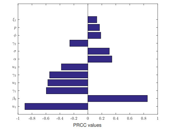
S. Marino, I. B. Hogue, C. J. Ray, D. E. Kirschner, A methodology for performing global uncertainty and sensitivity analysis in systems biology, J. Theor. Biol., 254 (2008), 178-196. doi: 10.1016/j.jtbi.2008.04.011
    [60] M. Z. Ndii, B. S. Djahi, N. D. Rumlaklak, A. K. Supriatna, Determining the important parameters of mathematical models of the propagation of malware, in: M. A. Othman, M. Z. A. Abd Aziz, M. S. Md Saat, M. H. Misran (Eds.), Proceedings of the 3rd International Symposium of Information and Internet Technology (SYMINTECH 2018), Springer International Publishing, Cham, 2019, pp. 1-9.
    [61] S. Lenhart, J. T. & Workman Optimal control applied to biological models. CRC Press, 2007.
  • This article has been cited by:

    1. M A A Pratama, A K Supriatna, N Anggriani, A mathematical model to study the effect of travel between two regions on the COVID-19 infections, 2021, 1722, 1742-6588, 012044, 10.1088/1742-6596/1722/1/012044
    2. A Islamilova, D Aldila, W Giyarti, H Tasman, Modelling the spread of atherosclerosis considering relapse and linear treatment, 2021, 1722, 1742-6588, 012039, 10.1088/1742-6596/1722/1/012039
    3. M. Fatimah, D. Aldila, B. D. Handari, Backward bifurcation arises from the smoking transmission model considering media campaign, 2021, 1722, 1742-6588, 012004, 10.1088/1742-6596/1722/1/012004
    4. Akhil Kumar Srivastav, Pankaj Kumar Tiwari, Prashant K Srivastava, Mini Ghosh, Yun Kang, A mathematical model for the impacts of face mask, hospitalization and quarantine on the dynamics of COVID-19 in India: deterministic vs. stochastic, 2021, 18, 1551-0018, 182, 10.3934/mbe.2021010
    5. Dipo Aldila, Analyzing the impact of the media campaign and rapid testing for COVID-19 as an optimal control problem in East Java, Indonesia, 2020, 141, 09600779, 110364, 10.1016/j.chaos.2020.110364
    6. Dipo Aldila, Besya Raisna Saslia, Wed Gayarti, Hengki Tasman, Backward bifurcation analysis on Tuberculosis disease transmission with saturated treatment, 2021, 1821, 1742-6588, 012002, 10.1088/1742-6596/1821/1/012002
    7. Akhil Kumar Srivastav, Mini Ghosh, Shraddha Ramdas Bandekar, Modeling of COVID-19 with limited public health resources: a comparative study of three most affected countries, 2021, 136, 2190-5444, 10.1140/epjp/s13360-021-01333-y
    8. Dipo Aldila, Brenda M. Samiadji, Gracia M. Simorangkir, Sarbaz H. A. Khosnaw, Muhammad Shahzad, Impact of early detection and vaccination strategy in COVID-19 eradication program in Jakarta, Indonesia, 2021, 14, 1756-0500, 10.1186/s13104-021-05540-9
    9. Dipo Aldila, Michellyn Angelina, Optimal control problem and backward bifurcation on malaria transmission with vector bias, 2021, 7, 24058440, e06824, 10.1016/j.heliyon.2021.e06824
    10. Ahmed S. Elgazzar, Simple mathematical models for controlling COVID-19 transmission through social distancing and community awareness, 2021, 0, 1865-7125, 10.1515/znc-2021-0004
    11. A. Mhlanga, T. V. Mupedza, A patchy theoretical model for the transmission dynamics of SARS-Cov-2 with optimal control, 2022, 12, 2045-2322, 10.1038/s41598-022-21553-1
    12. Hana Mutia Dewi, Ratna Herdiana, Priyo S. Sasongko, 2023, 2540, 0094-243X, 080014, 10.1063/5.0105905
    13. James Nicodemus Paul, Silas Steven Mirau, Isambi Sailon Mbalawata, Murat Sari, Mathematical Approach to Investigate Stress due to Control Measures to Curb COVID-19, 2022, 2022, 1748-6718, 1, 10.1155/2022/7772263
    14. Meksianis Z. Ndii, The effects of vaccination, vector controls and media on dengue transmission dynamics with a seasonally varying mosquito population, 2022, 34, 22113797, 105298, 10.1016/j.rinp.2022.105298
    15. Abadi Abay Gebremeskel, Hailay Weldegiorgis Berhe, Adugna Temesgen Abay, Kamal Shah, A Mathematical Modelling and Analysis of COVID-19 Transmission Dynamics with Optimal Control Strategy, 2022, 2022, 1748-6718, 1, 10.1155/2022/8636530
    16. Zenebe Shiferaw Kifle, Legesse Lemecha Obsu, Mathematical modeling for COVID-19 transmission dynamics: A case study in Ethiopia, 2022, 34, 22113797, 105191, 10.1016/j.rinp.2022.105191
    17. Jilan Alya, Dipo Aldila, Rahmi Rusin, 2022, 2501, 0094-243X, 020016, 10.1063/5.0082709
    18. Luis Vargas Tamayo, Vianney Mbazumutima, Christopher Thron, Léonard Todjihounde, Three-Stage Numerical Solution for Optimal Control of COVID-19, 2021, 9, 2227-7390, 1777, 10.3390/math9151777
    19. Shraddha Ramdas Bandekar, Mini Ghosh, Mathematical modeling of COVID-19 in India and its states with optimal control, 2022, 8, 2363-6203, 2019, 10.1007/s40808-021-01202-8
    20. Bo Wang, Jayanta Mondal, Piu Samui, Amar Nath Chatterjee, Abdullahi Yusuf, Effect of an antiviral drug control and its variable order fractional network in host COVID-19 kinetics, 2022, 231, 1951-6355, 1915, 10.1140/epjs/s11734-022-00454-4
    21. Endang Yuliani, Cicik Alfiniyah, Maureen L. Juga, Chidozie W. Chukwu, On the Modeling of COVID-19 Transmission Dynamics with Two Strains: Insight through Caputo Fractional Derivative, 2022, 6, 2504-3110, 346, 10.3390/fractalfract6070346
    22. G. Simorangkir, D. Aldila, A. Rizka, H. Tasman, E. S. Nugraha, Mathematical model of tuberculosis considering observed treatment and vaccination interventions, 2021, 24, 0972-0502, 1717, 10.1080/09720502.2021.1958515
    23. Shinta A. Rahmayani, Dipo Aldila, Bevina D. Handari, Cost-effectiveness analysis on measles transmission with vaccination and treatment intervention, 2021, 6, 2473-6988, 12491, 10.3934/math.2021721
    24. Justin M. Calabrese, Jeffery Demers, How optimal allocation of limited testing capacity changes epidemic dynamics, 2022, 538, 00225193, 111017, 10.1016/j.jtbi.2022.111017
    25. Benny Yong, Jonathan Hoseana, Livia Owen, From pandemic to a new normal: Strategies to optimise governmental interventions in Indonesia based on an SVEIQHR-type mathematical model, 2022, 7, 24680427, 346, 10.1016/j.idm.2022.06.004
    26. Utriweni Mukhaiyar, Kurnia Novita Sari, Yuli Sri Afrianti, Andi Muhammad Rinaldi Saputra, 2022, 2501, 0094-243X, 020022, 10.1063/5.0082756
    27. Dipo Aldila, Optimal control for dengue eradication program under the media awareness effect, 2021, 0, 1565-1339, 10.1515/ijnsns-2020-0142
    28. Dipo Aldila, Meksianis Z. Ndii, Nursanti Anggriani, Hengki Tasman, Bevina D. Handari, Impact of social awareness, case detection, and hospital capacity on dengue eradication in Jakarta: A mathematical model approach, 2023, 64, 11100168, 691, 10.1016/j.aej.2022.11.032
    29. Dipo Aldila, Bapan Ghosh, Dynamical Analysis on a Malaria Model with Relapse Preventive Treatment and Saturated Fumigation, 2022, 2022, 1748-6718, 1, 10.1155/2022/1135452
    30. M. Syamsurrijal, Achmad Nurmandi, Hasse Jubba, Mega Hidayati, Zuly Qodir, 2021, Chapter 27, 978-3-030-90178-3, 207, 10.1007/978-3-030-90179-0_27
    31. Novendra Setyawan, Tri Septiana Nadia Puspita Putri, Mohamad Al Fikih, Nur Kasan, 2021, Comparative Study of CNN and YOLOv3 in Public Health Face Mask Detection, 978-623-6264-20-1, 354, 10.23919/EECSI53397.2021.9624247
    32. Mayowa M. Ojo, Temitope O. Benson, Olumuyiwa James Peter, Emile Franc Doungmo Goufo, Nonlinear optimal control strategies for a mathematical model of COVID-19 and influenza co-infection, 2022, 607, 03784371, 128173, 10.1016/j.physa.2022.128173
    33. Muhammad Abdurrahman Rois, Cicik Alfiniyah, Chidozie W. Chukwu, Dynamic analysis and optimal control of COVID-19 with comorbidity: A modeling study of Indonesia, 2023, 8, 2297-4687, 10.3389/fams.2022.1096141
    34. H. Husnulkhotimah, R. Rusin, D. Aldila, 2021, 2374, 0094-243X, 030004, 10.1063/5.0058692
    35. P. K. Santra, D. Ghosh, G. S. Mahapatra, Ebenezer Bonyah, Chung-Min Liao, Mathematical Analysis of Two Waves of COVID-19 Disease with Impact of Vaccination as Optimal Control, 2022, 2022, 1748-6718, 1, 10.1155/2022/2684055
    36. Ihtisham Ul Haq, Nigar Ali, Hijaz Ahmad, Taher A. Nofal, On the fractional-order mathematical model of COVID-19 with the effects of multiple non-pharmaceutical interventions, 2022, 7, 2473-6988, 16017, 10.3934/math.2022877
    37. Bevina D. Handari, Dipo Aldila, Bunga O. Dewi, Hanna Rosuliyana, Sarbaz H. A. Khosnaw, Analysis of yellow fever prevention strategy from the perspective of mathematical model and cost-effectiveness analysis, 2021, 19, 1551-0018, 1786, 10.3934/mbe.2022084
    38. reza Najarzadeh, maryam dehghani, mohammad hassan asemani, roozbeh abolpour, Optimal Robust LPV Control Design for Novel Covid-19 Disease, 2021, 14, 2008-8345, 141, 10.52547/joc.14.5.141
    39. Elenice Weber Stiegelmeier, Glaucia Maria Bressan, A fuzzy approach in the study of COVID-19 pandemic in Brazil, 2021, 37, 2446-4732, 263, 10.1007/s42600-021-00144-5
    40. Meksianis Z. Ndii, Nursanti Anggriani, Jakobis J. Messakh, Bertha S. Djahi, Estimating the reproduction number and designing the integrated strategies against dengue, 2021, 27, 22113797, 104473, 10.1016/j.rinp.2021.104473
    41. Zenebe Shiferaw Kifle, Legesse Lemecha Obsu, Optimal control analysis of a COVID-19 model, 2023, 31, 2769-0911, 10.1080/27690911.2023.2173188
    42. Meksianis Z. Ndii, Yudi Ari Adi, Understanding the effects of individual awareness and vector controls on malaria transmission dynamics using multiple optimal control, 2021, 153, 09600779, 111476, 10.1016/j.chaos.2021.111476
    43. Rajanish Kumar Rai, Pankaj Kumar Tiwari, Subhas Khajanchi, Modeling the influence of vaccination coverage on the dynamics of COVID‐19 pandemic with the effect of environmental contamination, 2023, 0170-4214, 10.1002/mma.9185
    44. Suyalatu Dong, Linlin Xu, Yana A, Zhong-Zhou Lan, Ding Xiao, Bo Gao, Application of a time-delay SIR model with vaccination in COVID-19 prediction and its optimal control strategy, 2023, 0924-090X, 10.1007/s11071-023-08308-x
    45. Hailay Weldegiorgis Berhe, Abadi Abay Gebremeskel, Zinabu Teka Melese, Mo’tassem Al-arydah, Asdenaki Aklilu Gebremichael, Modeling and global stability analysis of COVID-19 dynamics with optimal control and cost-effectiveness analysis, 2024, 11, 26668181, 100843, 10.1016/j.padiff.2024.100843
    46. Shewafera Wondimagegnhu Teklu, Yohannes Fissha Abebaw, Birhanu Baye Terefe, Dejen Ketema Mamo, HIV/AIDS and TB co-infection deterministic model bifurcation and optimal control analysis, 2023, 41, 23529148, 101328, 10.1016/j.imu.2023.101328
    47. Raheleh Khanduzi, Amin Jajarmi, Asiyeh Ebrahimzadeh, Mehdi Shahini, A novel collocation method with a coronavirus optimization algorithm for the optimal control of COVID-19: A case study of Wuhan, China, 2024, 178, 00104825, 108680, 10.1016/j.compbiomed.2024.108680
    48. Tanuja Das, Shraddha Ramdas Bandekar, Akhil Kumar Srivastav, Prashant K Srivastava, Mini Ghosh, Role of immigration and emigration on the spread of COVID-19 in a multipatch environment: a case study of India, 2023, 13, 2045-2322, 10.1038/s41598-023-37192-z
    49. Yanbin Du, Hua Zhou, Research on safety strategies for nucleic acid testing in sudden epidemic conditions based on a SEIARD dynamic model, 2024, 14, 2045-2322, 10.1038/s41598-024-71595-w
    50. Mira Oktafiana, Widowati Widowati, Titi Udjiani, K. Kartono, R. H. S. Utomo, 2024, 3165, 0094-243X, 030007, 10.1063/5.0216954
    51. Jiamin Hu, Lu-Xing Yang, Xiaofan Yang, Kaifan Huang, Gang Li, Yong Xiang, Cost-Effective Company Response Policy for Product Co-Creation in Company-Sponsored Online Community, 2024, 54, 2168-2216, 4494, 10.1109/TSMC.2024.3379408
    52. Alberto d'Onofrio, Mimmo Iannelli, Piero Manfredi, Gabriela Marinoschi, Epidemic control by social distancing and vaccination: Optimal strategies and remarks on the COVID-19 Italian response policy, 2024, 21, 1551-0018, 6493, 10.3934/mbe.2024283
    53. Shafira Meiria Rahmasari, Ratna Herdiana, 2023, 2760, 0094-243X, 020015, 10.1063/5.0140163
    54. Rizki Chika Audita Ariyani, R. Heru Tjahjana, R. Heri Soelistyo Utomo, R. Isnanto, B. Warsito, Analysis Of Local Stability Of The Model On COVID-19 Spread In DKI Jakarta Province, 2023, 448, 2267-1242, 05006, 10.1051/e3sconf/202344805006
    55. Giulio Pisaneschi, Matteo Tarani, Giovanni Di Donato, Alberto Landi, Marco Laurino, Piero Manfredi, Optimal social distancing in epidemic control: cost prioritization, adherence and insights into preparedness principles, 2024, 14, 2045-2322, 10.1038/s41598-024-54955-4
    56. Sonu Lamba, Tanuja Das, Prashant K. Srivastava, Impact of infectious density-induced additional screening and treatment saturation on COVID-19: Modeling and cost-effective optimal control, 2024, 9, 24680427, 569, 10.1016/j.idm.2024.03.002
    57. Peng 鹏 Yang 杨, Ruguo 如国 Fan 范, Yibo 奕博 Wang 王, Yingqing 应青 Zhang 张, Dynamic analysis of major public health emergency transmission considering the dual-layer coupling of community–resident complex networks, 2024, 33, 1674-1056, 070206, 10.1088/1674-1056/ad39c7
    58. Iffatricia Haura Febiriana, Dipo Aldila, Bevina Desjwiandra Handari, Puji Budi Setia Asih, Muhamad Hifzhudin Noor Aziz, Exploring the Interplay Between Social Awareness and the Use of Bed Nets in a Malaria Control Program, 2024, 6, 25889338, 196, 10.1016/j.jobb.2024.06.005
    59. Shewafera Wondimagegnhu Teklu, Yohannes Fissha Abebaw, Ewa Pawluszewicz, Analysis of the HBV and TB Coinfection Model With Optimal Control Strategies and Cost‐Effectiveness, 2024, 2024, 1026-0226, 10.1155/2024/8811930
    60. Steven D. Silver, Pauline van den Driessche, Subhas Khajanchi, A dynamic multistate and control model of the COVID-19 pandemic, 2023, 2198-1833, 10.1007/s10389-023-02014-z
    61. Muhammad Abdurrahman Rois, Cicik Alfiniyah, Santi Martini, Dipo Aldila, Farai Nyabadza, Modeling and optimal control of COVID-19 with comorbidity and three-dose vaccination in Indonesia, 2024, 6, 25889338, 181, 10.1016/j.jobb.2024.06.004
    62. Abdurkadir Edeo Gemeda, Legesse Lemecha Obsu, Eshetu Dadi Gurmu, Shambel Tadesse Degefa, Mathematical modeling of tuberculosis transmission dynamics with vaccination and two lines of treatments: a caputo fractional approach, 2024, 1598-5865, 10.1007/s12190-024-02308-9
    63. Tsega Kahsay Gebretekle, Casper Albers, Martial L Ndeffo-Mbah, Modelling the impact of behavioural interventions during pandemics: A systematic review, 2025, 20, 1932-6203, e0310611, 10.1371/journal.pone.0310611
  • Reader Comments
  • © 2020 the Author(s), licensee AIMS Press. This is an open access article distributed under the terms of the Creative Commons Attribution License (http://creativecommons.org/licenses/by/4.0)
通讯作者: 陈斌, bchen63@163.com
  • 1. 

    沈阳化工大学材料科学与工程学院 沈阳 110142

  1. 本站搜索
  2. 百度学术搜索
  3. 万方数据库搜索
  4. CNKI搜索

Metrics

Article views(7324) PDF downloads(422) Cited by(63)

Other Articles By Authors

/

DownLoad:  Full-Size Img  PowerPoint
Return
Return

Catalog