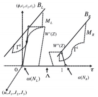
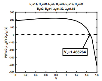
We study a quasi-one-dimensional steady-state Poisson-Nernst-Planck type model for ionic flows through a membrane channel with three ion species, two positively charged with the same valence and one negatively charged. Bikerman's local hard-sphere potential is included in the model to account for ion sizes. The problem is treated as a boundary value problem of a singularly perturbed differential system. Under the framework of a geometric singular perturbation theory, together with specific structures of this concrete model, the existence and uniqueness of solutions to the boundary value problem for small ion sizes is established. Furthermore, treating the ion sizes as small parameters, we derive an approximation of individual fluxes, from which one can further study the qualitative properties of ionic flows and extract concrete information directly related to biological measurements. Of particular interest is the competition between two cations due to the nonlinear interplay between finite ion sizes, diffusion coefficients and boundary conditions, which is closely related to selectivity phenomena of open ion channels with given protein structures. Furthermore, we are able to characterize the distinct effects of the nonlinear interplays between these physical parameters. Numerical simulations are performed to identify some critical potentials which play critical roles in examining properties of ionic flows in our analysis.
Citation: Peter W. Bates, Jianing Chen, Mingji Zhang. Dynamics of ionic flows via Poisson-Nernst-Planck systems with local hard-sphere potentials: Competition between cations[J]. Mathematical Biosciences and Engineering, 2020, 17(4): 3736-3766. doi: 10.3934/mbe.2020210
We study a quasi-one-dimensional steady-state Poisson-Nernst-Planck type model for ionic flows through a membrane channel with three ion species, two positively charged with the same valence and one negatively charged. Bikerman's local hard-sphere potential is included in the model to account for ion sizes. The problem is treated as a boundary value problem of a singularly perturbed differential system. Under the framework of a geometric singular perturbation theory, together with specific structures of this concrete model, the existence and uniqueness of solutions to the boundary value problem for small ion sizes is established. Furthermore, treating the ion sizes as small parameters, we derive an approximation of individual fluxes, from which one can further study the qualitative properties of ionic flows and extract concrete information directly related to biological measurements. Of particular interest is the competition between two cations due to the nonlinear interplay between finite ion sizes, diffusion coefficients and boundary conditions, which is closely related to selectivity phenomena of open ion channels with given protein structures. Furthermore, we are able to characterize the distinct effects of the nonlinear interplays between these physical parameters. Numerical simulations are performed to identify some critical potentials which play critical roles in examining properties of ionic flows in our analysis.

| [1] |
N. Abaid, R. S. Eisenberg, W. Liu, Asymptotic expansions of I-V relations via a Poisson-NernstPlanck system, SIAM J. Appl. Dyn. Syst., 7 (2008), 1507-1526. doi: 10.1137/070691322

|
| [2] |
R. Aitbayev, P. W. Bates, H. Lu, L. Zhang, M. Zhang, Mathematical studies of Poisson-NernstPlanck systems: dynamics of ionic flows without electroneutrality conditions, J. Comput. Appl. Math., 362 (2019), 510-527. doi: 10.1016/j.cam.2018.10.037
|
| [3] |
V. Barcilon, Ion flow through narrow membrane channels: Part I, SIAM J. Appl. Math., 52 (1992), 1391-1404. doi: 10.1137/0152080
|
| [4] |
V. Barcilon, D. P. Chen, R. S. Eisenberg, Ion flow through narrow membrane channels: Part II, SIAM J. Appl. Math., 52 (1992), 1405-1425. doi: 10.1137/0152081
|
| [5] |
V. Barcilon, D. P. Chen, R. S. Eisenberg, J. W. Jerome, Qualitative properties of steady-state Poisson-Nernst-Planck systems: Perturbation and simulation study, SIAM J. Appl. Math., 57 (1997), 631-648. doi: 10.1137/S0036139995312149
|
| [6] | P. W. Bates, Y. Jia, G. Lin, H. Lu, M. Zhang, Individual flux study via steady-state PoissonNernst-Planck systems: Effects from boundary conditions, SIAM J. Appl. Dyn. Syst., 16 (2017), |
| [7] |
P. W. Bates, W. Liu, H. Lu, M. Zhang, Ion size and valence effects on ionic flows via PoissonNernst-Planck models, Commu. Math. Sci., 15 (2017), 881-901. doi: 10.4310/CMS.2017.v15.n4.a1
|
| [8] |
J. J. Bikerman, Structure and capacity of the electrical double layer, Philos. Mag. J. Sci., 33 (1942), 384-397. doi: 10.1080/14786444208520813
|
| [9] |
D. Boda, D. Busath, B. Eisenberg, D. Henderson, W. Nonner, Monte Carlo simulations of ion selectivity in a biological Na+ channel: Charge-space competition, Phys. Chem. Chem. Phys., 4 (2002), 5154-5160. doi: 10.1039/B203686J
|
| [10] | D. Boda, D. Gillespie, W. Nonner, D. Henderson, B. Eisenberg, Computing induced charges in inhomogeneous dielectric media: Application in a Monte Carlo simulation of complex ionic systems, Phys. Rev. E, 69 (2004), 046702. |
| [11] |
D. Boda, W. Nonner, M. Valiskó, D. Henderson, B. Eisenberg, D. Gillespie, Steric selectivity in Na+ channels arising from protein polarization and mobile side chains, Biophys J., 93 (2007), 1960-1980. doi: 10.1529/biophysj.107.105478
|
| [12] |
D. Boda, W. Nonner, D. Henderson, B. Eisenberg, D. Gillespie, Volume exclusion in calcium selective channels, Biophys J., 94 (2008), 3486-3496. doi: 10.1529/biophysj.107.122796
|
| [13] |
M. Burger, R. S. Eisenberg, H. W. Engl, Inverse problems related to ion channel selectivity, SIAM J. Appl. Math., 67 (2007), 960-989. doi: 10.1137/060664689
|
| [14] |
A. E. Cardenas, R. D. Coalson, M. G. Kurnikova, Three-Dimensional Poisson-Nernst-Planck Theory Studies: Influence of Membrane Electrostatics on Gramicidin A Channel Conductance, Biophys. J., 79 (2000), 80-93. doi: 10.1016/S0006-3495(00)76275-8
|
| [15] |
J. H. Chaudhry, S. D. Bond, L. N. Olson, Finite Element Approximation to a Finite-Size Modified Poisson-Boltzmann Equation, J. Sci. Comput., 47 (2011), 347-364. doi: 10.1007/s10915-010-9441-7
|
| [16] | D. P. Chen, R. S. Eisenberg, Charges, currents and potentials in ionic channels of one conformation, Biophys. J., 64 (1993), 1405-1421. |
| [17] |
S. Chung, S. Kuyucak, Predicting channel function from channel structure using Brownian dynamics simulations, Clin. Exp. Pharmacol Physiol., 28 (2001), 89-94. doi: 10.1046/j.1440-1681.2001.03408.x
|
| [18] |
J. R. Clay, Potassium current in the squid giant axon, Int. Rev. Neurobiol., 27 (1985), 363-384. doi: 10.1016/S0074-7742(08)60562-0
|
| [19] |
R. Coalson, M. Kurnikova, Poisson-Nernst-Planck theory approach to the calculation of current through biological ion channels, IEEE Trans. NanoBioscience, 4 (2005), 81-93. doi: 10.1109/TNB.2004.842495
|
| [20] |
B. Corry, T. W. Allen, S. Kuyucak, S. H. Chung, Mechanisms of permeation and selectivity in calcium channels, Biophys J., 80 (2001), 195-214. doi: 10.1016/S0006-3495(01)76007-9
|
| [21] | B. Corry, T. W. Allen, S. Kuyucak, S. H. Chung, A model of calcium channels, Biochim. Biophys. Acta Biomembr., 1509 (2000), 1-6. |
| [22] |
B. Corry, S. H. Chung, Mechanisms of valence selectivity in biological ion channels, Cell. Mol. Life Sci., 63 (2006), 301-315. doi: 10.1007/s00018-005-5405-8
|
| [23] |
J. M. Diamond, E. M. Wright, Biological membranes: the physical basis of ion and nonelectrolyte selectivity, Annu. Rev. Physiol., 31 (1969), 581-646. doi: 10.1146/annurev.ph.31.030169.003053
|
| [24] | D. A. Doyle, J. M. Cabral, R. A. Pfuetzner, A. Kuo, J. M. Gulbis, S. L. Cohen, et al., The Structure of the Potassium Channel: Molecular Basis of K+ Conduction and Selectivity, Science, 280 (1998), 69-77. |
| [25] |
R. Dutzler, E. B. Campbell, M. Cadene, B. T. Chait, R. Mackinnon, X-ray structure of a ClC chloride channel at 3.0 A reveals the molecular basis of anion selectivity, Nature, 415 (2002), 287-294. doi: 10.1038/415287a
|
| [26] |
R. Dutzler, E.B. Campbell, R. MacKinnon, Gating the selectivity filter in ClC chloride channels, Science, 300 (2003), 108-112. doi: 10.1126/science.1082708
|
| [27] | B. Eisenberg, Ion Channels as Devices, J. Comput. Electron., 2 (2003), 245-249. |
| [28] | B. Eisenberg, Proteins, Channels, and Crowded Ions, Biophys. Chem., 100 (2003), 507-517. |
| [29] | R. S. Eisenberg, Channels as enzymes, J. Memb. Biol., 115 (1990), 1-12. |
| [30] | R. S. Eisenberg, R. Elber, Atomic biology, electrostatics and Ionic Channels, in New Developments and Theoretical Studies of Proteins, World Scientific, (1996), 269-357. |
| [31] |
R. S. Eisenberg, From Structure to Function in Open Ionic Channels, J. Memb. Biol., 171 (1999), 1-24. doi: 10.1007/s002329900554
|
| [32] |
B. Eisenberg, W. Liu, Poisson-Nernst-Planck systems for ion channels with permanent charges, SIAM J. Math. Anal., 38 (2007), 1932-1966. doi: 10.1137/060657480
|
| [33] |
G. Eisenman, R. Horn, Ionic selectivity revisited: The role of kinetic and equilibrium processes in ion permeation through channels, J. Memb. Biol., 76 (1983), 197-225. doi: 10.1007/BF01870364
|
| [34] |
A. Ern, R. Joubaud, T. Leliévre, Mathematical study of non-ideal electrostatic correlations in equilibrium electrolytes, Nonlinearity, 25 (2012), 1635-1652. doi: 10.1088/0951-7715/25/6/1635
|
| [35] |
N. Fenichel, Geometric singular perturbation theory for ordinary differential equations, J. Differ. Equations, 31 (1979), 53-98. doi: 10.1016/0022-0396(79)90152-9
|
| [36] |
D. Fertig, B. Matejczyk, M. Valiskó, D. Gillespie, D. Boda, Scaling Behavior of Bipolar Nanopore Rectification with Multivalent Ions, J. Phys. Chem. C., 123 (2019), 28985-28996. doi: 10.1021/acs.jpcc.9b07574
|
| [37] | J. Fischer, U. Heinbuch, Relationship between free energy density functional, Born-Green-Yvon, and potential distribution approaches for inhomogeneous fluids, J. Chem. Phys., 88 (1988), 1909-1913. |
| [38] | T. Gamble, K. Decker, T. S Plett, M. Pevarnik, J.F. Pietschmann, I. V. Vlassiouk, et al., Rectification of ion current in nanopores depends on the type of monovalent cations-experiments and modeling, J. Phys. Chem. C, 118 (2014), 9809-9819. |
| [39] | D. Gillespie, A singular perturbation analysis of the Poisson-Nernst-Planck system: Applications to Ionic Channels, Ph. D Dissertation, Rush University, Chicago, 1999. |
| [40] |
D. Gillespie, R. S. Eisenberg, Physical descriptions of experimental selectivity measurements in ion channels, European Biophys. J., 31 (2002), 454-466. doi: 10.1007/s00249-002-0239-x
|
| [41] |
D. Gillespie, W. Nonner, R. S. Eisenberg, Coupling Poisson-Nernst-Planck and density functional theory to calculate ion flux, J. Phys. Condens. Matter, 14 (2002), 12129-12145. doi: 10.1088/0953-8984/14/46/317
|
| [42] | D. Gillespie, W. Nonner, R. S. Eisenberg, Density functional theory of charged, hard-sphere fluids, Phys. Rev. E, 68 (2003), 0313503. |
| [43] | D. Gillespie, W. Nonner, R. S. Eisenberg, Crowded Charge in Biological Ion Channels, Nanotech, 3 (2003), 435-438. |
| [44] | E. Gongadze, U. van Rienen, V. Kralj-lglič, A. lglič, Spatial variation of permittivity of an electrolyte solution in contact with a charged metal surface: A mini review, Comput. Method Biomech. Biomed. Eng., 16 (2013), 463-480. |
| [45] | B. Hille, Ionic Channels of Excitable Membranes, Sinauer Associates Inc, (2001). |
| [46] | B. Hille, Ionic Selectivity, saturation, and block in sodium channels. A four barrier model, J. Gen. Physiol., 66 (1975), 535-560. |
| [47] | U. Hollerbach, D. P. Chen, R. S. Eisenberg, Two- and Three-Dimensional Poisson-Nernst-Planck Simulations of Current Flow through Gramicidin-A, J. Comp. Science, 16 (2002), 373-409. |
| [48] | U. Hollerbach, D. Chen, W. Nonner, B. Eisenberg, Three-dimensional Poisson-Nernst-Planck Theory of Open Channels, Biophys. J., 76 (1999), A205. |
| [49] | A. L. Hodgkin, The Conduction of the Nervous Impulse, Liverpool University Press, (1971), 1-108. |
| [50] | A. L. Hodgkin, Chance and Design, Cambridge University Press, (1992). |
| [51] |
A. L. Hodgkin, A. F. Huxley, Propagation of electrical signals along giant nerve fibres, Proc. R. Soc. London B, 140 (1952), 177-183. doi: 10.1098/rspb.1952.0054
|
| [52] |
A. L. Hodgkin, A. F. Huxley, Currents carried by sodium and potassium ions through the membrane of the giant axon of Loligo, J. Physiol., 116 (1952), 449-472. doi: 10.1113/jphysiol.1952.sp004717
|
| [53] |
A. L. Hodgkin, A. F. Huxley, The components of membrane conductance in the giant axon of Loligo, J. Physiol., 116 (1952), 473-496. doi: 10.1113/jphysiol.1952.sp004718
|
| [54] |
A. L. Hodgkin, A. F. Huxley, The dual effect of membrane potential on sodium conductance in the giant axon of Loligo, J. Physiol., 116 (1952), 497-506. doi: 10.1113/jphysiol.1952.sp004719
|
| [55] |
A. L. Hodgkin, A. F. Huxley, A quantitive description of membrane current and its application to conduction and excitation in nerve, J. Physiol., 117 (1952), 500-544. doi: 10.1113/jphysiol.1952.sp004764
|
| [56] | Y. Hyon, B. Eisenberg, C. Liu, A mathematical model for the hard sphere repulsion in ionic solutions, Commun. Math. Sci., 9 (2010), 459-475. |
| [57] |
Y. Hyon, J. Fonseca, B. Eisenberg, C. Liu, Energy variational approach to study charge inversion (layering) near charged walls, Discrete Contin. Dyn. Syst. B, 17 (2012), 2725-2743. doi: 10.3934/dcdsb.2012.17.2725
|
| [58] |
Y. Hyon, C. Liu, B. Eisenberg, PNP equations with steric effects: a model of ion flow through channels, J. Phys. Chem. B, 116 (2012), 11422-11441. doi: 10.1021/jp305273n
|
| [59] |
W. Im, D. Beglov, B. Roux, Continuum solvation model: Electrostatic forces from numerical solutions to the Poisson-Bolztmann equation, Comp. Phys. Comm., 111 (1998), 59-75. doi: 10.1016/S0010-4655(98)00016-2
|
| [60] | W. Im, B. Roux, Ion permeation and selectivity of OmpF porin: A theoretical study based on molecular dynamics, Brownian dynamics, and continuum electrodiffusion theory, J. Mol. Biol., 322 (2002), 851-869. |
| [61] |
S. Ji, W. Liu, Poisson-Nernst-Planck Systems for Ion Flow with Density Functional Theory for Hard-Sphere Potential: I-V relations and Critical Potentials. Part I: Analysis, J. Dyn. Diff. Equat., 24 (2012), 955-983. doi: 10.1007/s10884-012-9277-y
|
| [62] |
S. Ji, W. Liu, M. Zhang, Effects of (small) permanent charges and channel geometry on ionic flows via classical Poisson-Nernst-Planck models, SIAM J. on Appl. Math., 75 (2015), 114-135. doi: 10.1137/140992527
|
| [63] |
Y. Jia, W. Liu, M. Zhang, Qualitative properties of ionic flows via Poisson-Nernst-Planck systems with Bikerman's local hard-sphere potential: Ion size effects, Discrete Contin. Dyn. Syst. B, 21 (2016), 1775-1802. doi: 10.3934/dcdsb.2016022
|
| [64] | C. Jones, Geometric singular perturbation theory, in Dynamical systems, Springer, (1995), 44-118. |
| [65] |
C. Jones, T. Kaper, N. Kopell, Tracking invariant manifolds up to exponentially small errors, SIAM J. Math. Anal., 27 (1996), 558-577. doi: 10.1137/S003614109325966X
|
| [66] |
C. Jones, N. Kopell, Tracking invariant manifolds with differential forms in singularly perturbed systems, J. Differ. Equations, 108 (1994), 64-88. doi: 10.1006/jdeq.1994.1025
|
| [67] |
A. S. Khair, T. M. Squires, Ion steric effects on electrophoresis of a colloidal particle, J. Fluid Mech., 640 (2009), 343-356. doi: 10.1017/S0022112009991728
|
| [68] | M. S. Kilic, M. Z. Bazant, A. Ajdari, Steric effects in the dynamics of electrolytes at large applied voltages. II. Modified Poisson-Nernst-Planck equations, Phys. Rev. E, 75 (2007), 021503. |
| [69] |
C. C. Lee, H. Lee, Y. Hyon, T. C. Lin, C. Liu, New Poisson-Boltzmann type equations: Onedimensional solutions, Nonlinearity, 24 (2011), 431-458. doi: 10.1088/0951-7715/24/2/004
|
| [70] |
B. Li, Continuum electrostatics for ionic solutions with non-uniform ionic sizes, Nonlinearity, 22 (2009), 811-833. doi: 10.1088/0951-7715/22/4/007
|
| [71] |
G. Lin, W. Liu, Y. Yi, M. Zhang, Poisson-Nernst-Planck systems for ion flow with density functional theory for local hard-sphere potential, SIAM J. Appl. Dyn. Syst., 12 (2013), 1613-1648. doi: 10.1137/120904056
|
| [72] |
W. Liu, Geometric singular perturbation approach to steady-state Poisson-Nernst-Planck systems, SIAM J. Appl. Math., 65 (2005), 754-766. doi: 10.1137/S0036139903420931
|
| [73] |
W. Liu, One-dimensional steady-state Poisson-Nernst-Planck systems for ion channels with multiple ion species, J. Differ. Equations, 246 (2009), 428-451. doi: 10.1016/j.jde.2008.09.010
|
| [74] |
W. Liu, H. Xu, A complete analysis of a classical Poisson-Nernst-Planck model for ionic flow, J. Differ. Equations, 258 (2015), 1192-1228. doi: 10.1016/j.jde.2014.10.015
|
| [75] |
W. Liu, B. Wang, Poisson-Nernst-Planck systems for narrow tubular-like membrane channels, J. Dyn. Differ. Equations, 22 (2010), 413-437. doi: 10.1007/s10884-010-9186-x
|
| [76] |
W. Liu, X. Tu, M. Zhang, Poisson-Nernst-Planck Systems for Ion Flow with Density Functional Theory for Hard-Sphere Potential: I-V relations and Critical Potentials. Part II: Numerics, J. Dyn. Differ. Equations, 24 (2012), 985-1004. doi: 10.1007/s10884-012-9278-x
|
| [77] | H. Lu, J. Li, J. Shackelford, J. Vorenberg, M. Zhang, Ion size effects on individual fluxes via Poisson-Nernst-Planck systems with Bikerman's local hard-sphere potential: Analysis without electroneutrality boundary conditions, Discrete Contin. Dyn. Syst. B, 23 (2018), 1623-1643. |
| [78] | B. Matejczyk, M. Valiskó, M. T. Wolfram, J. F. Pietschmann, D. Boda, Multiscale modeling of a rectifying bipolar nanopore: Comparing Poisson-Nernst-Planck to Monte Carlo, J. Chem. Phys., 146 (2017), 124125. |
| [79] |
J. H. Morais-Cabral, Y. Zhou, R. MacKinnon, Energetic optimization of ion conduction rate by the K+ selectivity filter, Nature, 414 (2001), 37-42. doi: 10.1038/35102000
|
| [80] |
L. J. Mullins, Ion selectivity of carriers and channels, Biophys J., 15 (1975), 921-931. doi: 10.1016/S0006-3495(75)85867-X
|
| [81] | B. Nadler, Z. Schuss, A. Singer, B. Eisenberg, Diffusion through protein channels: from molecular description to continuum equations, Technical Proceedings of the Nanotechnology Conference and Trade Show, 2003. Available from: https: //ftp.rush.edu/. |
| [82] |
W. Nonner, R. S. Eisenberg, Ion permeation and glutamate residues linked by Poisson-NernstPlanck theory in L-type Calcium channels, Biophys. J., 75 (1998), 1287-1305. doi: 10.1016/S0006-3495(98)74048-2
|
| [83] |
S. Y. Noskov, W. Im, B. Roux, Ion Permeation through the z1-Hemolysin Channel: Theoretical Studies Based on Brownian Dynamics and Poisson-Nernst-Planck Electrodiffusion Theory, Biophys. J., 87 (2004), 2299-2309. doi: 10.1529/biophysj.104.044008
|
| [84] | S. Y. Noskov, B. Roux, Ion selectivity in potassium channels, Biophys. Chem., 124 (2006), 279-291. |
| [85] |
J. K. Park, J. W. Jerome, Qualitative properties of steady-state Poisson-Nernst-Planck systems: Mathematical study, SIAM J. Appl. Math., 57 (1997), 609-630. doi: 10.1137/S0036139995279809
|
| [86] |
J. K. Percus, Equilibrium state of a classical fluid of hard rods in an external field, J. Stat. Phys., 15 (1976), 505-511. doi: 10.1007/BF01020803
|
| [87] |
J. K. Percus, Model grand potential for a nonuniform classical fluid, J. Chem. Phys., 75 (1981), 1316-1319. doi: 10.1063/1.442136
|
| [88] |
Y. Qiao, X. Liu, M. Chen, B. Lu, A Local Approximation of Fundamental Measure Theory Incorporated into Three Dimensional Poisson-Nernst-Planck Equations to Account for Hard Sphere Repulsion Among Ions, J. Stat. Phys., 163 (2016), 156-174. doi: 10.1007/s10955-016-1470-7
|
| [89] | P. Ramirez, J. A. Manzanares, J. Cervera, V. Gomez, M. Ali, I. Pause, et al., Nanopore charge inversion and current-voltage curves in mixtures of asymmetric electrolytes, J. Membr. Sci., 563 (2018), 633-642. |
| [90] |
Y. Rosenfeld, Free-Energy Model for the Inhomogeneous Hard-Sphere Fluid Mixture and Density-Functional Theory of Freezing, Phys. Rev. Lett., 63 (1989), 980-983. doi: 10.1103/PhysRevLett.63.980
|
| [91] | Y. Rosenfeld, Free energy model for the inhomogeneous fluid mixtures: Yukawa-charged hard spheres, general interactions, and plasmas, J. Chem. Phys., 98 (1993), 8126-8148. |
| [92] | R. Roth, Fundamental measure theory for hard-sphere mixtures: A review, J. Phys. Condens. Matter, 22 (2010), 063102. |
| [93] |
B. Roux, T. W. Allen, S. Berneche, W. Im, Theoretical and computational models of biological ion channels, Quat. Rev. Biophys., 37 (2004), 15-103. doi: 10.1017/S0033583504003968
|
| [94] | D. Colquhoun, F. J. Sigworth, Single-Channel Recording, Plenum Press, (1995). |
| [95] | Z. Schuss, B. Nadler, R. S. Eisenberg, Derivation of Poisson and Nernst-Planck equations in a bath and channel from a molecular model, Phys. Rev. E, 64 (2001), 1-14. |
| [96] |
F. Siddiqua, Z. Wang, S. Zhou, A Modified Poisson-Nernst-Planck Model with Excluded Volume Effect: Theory and Numerical Implementation, Commun. Math. Sci., 16 (2018), 251-271. doi: 10.4310/CMS.2018.v16.n1.a12
|
| [97] |
A. Singer, D. Gillespie, J. Norbury, R. S. Eisenberg, Singular perturbation analysis of the steadystate Poisson-Nernst-Planck system: applications to ion channels, Eur. J. Appl. Math., 19 (2008), 541-560. doi: 10.1017/S0956792508007596
|
| [98] |
A. Singer, J. Norbury, A Poisson-Nernst-Planck model for biological ion channels-an asymptotic analysis in a three-dimensional narrow funnel, SIAM J. Appl. Math., 70 (2009), 949-968. doi: 10.1137/070687037
|
| [99] |
L. Sun, W. Liu, Non-localness of Excess Potentials and Boundary Value Problems of PoissonNernst-Planck Systems for Ionic Flow: A Case Study, J. Dyn. Differ. Equations, 30 (2018), 779-797. doi: 10.1007/s10884-017-9578-2
|
| [100] |
S. K. Tin, N. Kopell, C. Jones, Invariant manifolds and singularly perturbed boundary value problems, SIAM J. Numer. Anal., 31 (1994), 1558-1576. doi: 10.1137/0731081
|
| [101] | M. Valiskó, B. Matejczyk, Z. Ható, T. Kristóf, E. Mádai, D. Fertig, et al., Multiscale analysis of the effect of surface charge pattern on a nanopore's rectification and selectivity properties: from all-atom model to Poisson-Nernst-Planck, J. Chem. Phys., 150 (2019), 144703. |
| [102] | X. S. Wang, D. He, J. Wylie, H. Huang, Singular perturbation solutions of steady-state PoissonNernst-Planck systems, Phys. Rev. E, 89 (2014), 022722. |
| [103] |
G. W. Wei, Q. Zheng, Z. Chen, K. Xia, Variational multiscale models for charge transport, SIAM Rev., 54 (2012), 699-754. doi: 10.1137/110845690
|
| [104] | M. Zhang, Asymptotic expansions and numerical simulations of I-V relations via a steady-state Poisson-Nernst-Planck system, Rocky Mt. J. Math., 45 (2015), 1681-1708. |
| [105] |
M. Zhang, Boundary layer effects on ionic flows via classical Poisson-Nernst-Planck systems, Comput. Math. Biophys., 6 (2018), 14-27. doi: 10.1515/cmb-2018-0002
|
| [106] |
J. Zhang, D. Acheampong, M. Zhang, Effects on ionic flows from finite ion sizes via PoissonNernst-Planck models with non-local excess chemical potentials, Comput. Math. Biophys., 5 (2017), 58-77. doi: 10.1515/mlbmb-2017-0005
|
| [107] | Q. Zheng, G. W. Wei, Poisson-Boltzmann-Nernst-Planck model, J. Chem. Phys., 134 (2011), 194101. |
| [108] |
Y. Zhou, R. MacKinnon, The occupancy of ions in the K+ selectivity filter: charge balance and coupling of ion binding to a protein conformational change underlie high conduction rates, J. Mol. Biol., 333 (2003), 965-975. doi: 10.1016/j.jmb.2003.09.022
|
| [109] |
M. Zhou, R. MacKinnon, A mutant KcsA K+ channel with altered conduction properties and selectivity filter ion distribution, J. Mol. Biol., 338 (2004), 839-846. doi: 10.1016/j.jmb.2004.03.020
|

Figures(3)

Peter W. Bates, Jianing Chen, Mingji Zhang. Dynamics of ionic flows via Poisson-Nernst-Planck systems with local hard-sphere potentials: Competition between cations[J]. Mathematical Biosciences and Engineering, 2020, 17(4): 3736-3766. doi: 10.3934/mbe.2020210


 DownLoad: