Novel optical soliton solutions for the generalized integrable (2+1)- dimensional nonlinear Schrödinger system with conformable derivative

Muhammad Bilal; Javed Iqbal; Ikram Ullah; Aditi Sharma; Hasim Khan; Sunil Kumar Sharma; Muhammad Bilal; Javed Iqbal; Ikram Ullah; Aditi Sharma; Hasim Khan; Sunil Kumar Sharma

doi:10.3934/math.2025497

AIMS Mathematics

2025, Volume 10, Issue 5: 10943-10975. doi: 10.3934/math.2025497

Previous Article Next Article

Research article

Novel optical soliton solutions for the generalized integrable (2+1)- dimensional nonlinear Schrödinger system with conformable derivative

1.
Department of Mathematics, Abdul Wali Khan University, Mardan 23200, KPK, Pakistan
2.
School of Mathematics and Statistics, Central South University, Changsha 410083, Hunan, China
3.
Department of Computer Science and Engineering, Symbiosis Institute of Technology, Symbiosis International (Deemed University), Pune, India
4.
Department of Mathematics, College of Science, Jazan University, P. O. Box 114, Jazan 45142, Saudi Arabia
5.
Department of Information Systems College of Computer and Information Sciences Majmaah University, Majmaah 11952, Saudi Arabia

Received: 01 March 2025 Revised: 21 April 2025 Accepted: 27 April 2025 Published: 13 May 2025
MSC : 65F10, 65H10, 90C30, 90C33

For the generalized integrable (2+1)-dimensional nonlinear Schrödinger system, new and creative analytical solutions were derived using a novel extended direct algebraic method incorporating conformable derivatives, which could be expressed in terms of elementary functions and yielded a variety of analytical solutions, such as single, optical periodic, and wave solitons. The analytical solutions provided key insights into the effects of conformable derivatives and temporal parameters on the behavior of optical solitons, such as their stability, propagation, and interaction. To further elucidate the dynamics of these solitons, 2D, 3D, and contour plots were created to provide a visual representation of the soliton's form, amplitude, and phase. This helps to better understand the behavior of the soliton and its potential applications in nonlinear equations. Based on the study's demonstration of the extended direct algebraic method's strength and versatility in obtaining analytical solutions for complex non linear systems, it may be a useful tool for solving a variety of nonlinear problems in science and engineering.
- extended Direct algebraic approach,
- conformable derivatives,
- nonlinear system,
- analytical solutions,
- generalized integrable nonlinear Schrödinger system
Citation: Muhammad Bilal, Javed Iqbal, Ikram Ullah, Aditi Sharma, Hasim Khan, Sunil Kumar Sharma. Novel optical soliton solutions for the generalized integrable (2+1)- dimensional nonlinear Schrödinger system with conformable derivative[J]. AIMS Mathematics, 2025, 10(5): 10943-10975. doi: 10.3934/math.2025497

Related Papers:

Abstract

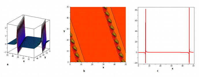
For the generalized integrable (2+1)-dimensional nonlinear Schrödinger system, new and creative analytical solutions were derived using a novel extended direct algebraic method incorporating conformable derivatives, which could be expressed in terms of elementary functions and yielded a variety of analytical solutions, such as single, optical periodic, and wave solitons. The analytical solutions provided key insights into the effects of conformable derivatives and temporal parameters on the behavior of optical solitons, such as their stability, propagation, and interaction. To further elucidate the dynamics of these solitons, 2D, 3D, and contour plots were created to provide a visual representation of the soliton's form, amplitude, and phase. This helps to better understand the behavior of the soliton and its potential applications in nonlinear equations. Based on the study's demonstration of the extended direct algebraic method's strength and versatility in obtaining analytical solutions for complex non linear systems, it may be a useful tool for solving a variety of nonlinear problems in science and engineering.

References

[1]	H. Yépez-Martínez, J. F. Gómez-Aguilar, A. Atangana, First integral method for non-linear differential equations with conformable derivative, Math. Model. Nat. Phenom., 13 (2018), 14. https://doi.org/10.1051/mmnp/2018012 doi: 10.1051/mmnp/2018012
[2]	H. Tajadodi, Z. A. Khan, A. ur R. Irshad, J. F. Gómez-Aguilar, A. Khan, H. Khan, Exact solutions of conformable fractional differential equations, Results Phys., 22 (2021), 103916. https://doi.org/10.1016/j.rinp.2021.103916 doi: 10.1016/j.rinp.2021.103916
[3]	S. R. Aderyani, R. Saadati, J. Vahidi, J. F. Gómez-Aguilar, The exact solutions of conformable time-fractional modified nonlinear Schrödinger equation by first integral method and functional variable method, Opt. Quant. Electron., 54 (2022), 218. https://doi.org/10.1007/s11082-022-03605-y doi: 10.1007/s11082-022-03605-y
[4]	H. Yépez-Martínez, A. Pashrashid, J. F. Gómez-Aguilar, L. Akinyemi, H. Rezazadeh, The novel soliton solutions for the conformable perturbed nonlinear Schrödinger equation, Mod. Phys. Lett. B, 36 (2022), 2150597. https://doi.org/10.1142/S0217984921505977 doi: 10.1142/S0217984921505977
[5]	K. Zhang, J. P. Cao, J. J. Lyu, Dynamic behavior and modulation instability for a generalized nonlinear Schrödinger equation with nonlocal nonlinearity, Phys. Scr., 100 (2024), 015262. https://doi.org/ 10.1088/1402-4896/ad9cfa doi: 10.1088/1402-4896/ad9cfa
[6]	Z. Li, J. J. Lyu, E. Hussain, Bifurcation, chaotic behaviors and solitary wave solutions for the fractional Twin-Core couplers with Kerr law non-linearity, Sci. Rep., 14 (2024), 22616. https://doi.org/10.1038/s41598-024-74044-w doi: 10.1038/s41598-024-74044-w
[7]	D. Chen, D. Shi, F. Chen, Qualitative analysis and new traveling wave solutions for the stochastic Biswas-Milovic equation, AIMS Mathematics, 10 (2025), 4092–4119. https://doi.org/10.3934/math.2025190 doi: 10.3934/math.2025190
[8]	Z. Li, S. Zhao, Bifurcation, chaotic behavior and solitary wave solutions for the Akbota equation, AIMS Mathematics, 9 (2024), 22590–22601. https://doi.org/10.3934/math.20241100 doi: 10.3934/math.20241100
[9]	A. R. Seadawy, M. Iqbal, Dispersive propagation of optical solitions and solitary wave solutions of Kundu-Eckhaus dynamical equation via modified mathematical method, Appl. Math. J. Chin. Univ., 38 (2023), 16–26. https://doi.org/10.1007/s11766-023-3861-2 doi: 10.1007/s11766-023-3861-2
[10]	W. A. Faridi, S. A. AlQahtani, The explicit power series solution formation and computationof Lie point infinitesimals generators: Lie symmetry approach, Phys. Scr., 98 (2023), 125249. https://doi.org/10.1088/1402-4896/ad0948 doi: 10.1088/1402-4896/ad0948
[11]	K. K. Ahmed, H. M. Ahmed, W. B. Rabie, M. F. Shehab, Effect of noise on wave solitons for (3+1)-dimensional nonlinear Schrödinger equation in optical fiber, Indian J. Phys., 98 (2024), 4863–4882. https://doi.org/10.1007/s12648-024-03222-3 doi: 10.1007/s12648-024-03222-3
[12]	A. M. Elsherbeny, A. Bekir, A. H. Arnous, M. Sadaf, G. Akram, Solitons to the time-fractional Radhakrishnan–Kundu–Lakshmanan equation with $\beta$ and M-truncated fractional derivatives: a comparative analysis, Opt. Quant. Electron., 55 (2023), 1112. https://doi.org/10.1007/s11082-023-05414-3 doi: 10.1007/s11082-023-05414-3
[13]	M. A. S. Murad, Analysis of time-fractional Schrödinger equation with group velocity dispersion coefficients and second-order spatiotemporal effects: a new Kudryashov approach, Opt. Quant. Electron., 56 (2024), 908. https://doi.org/10.1007/s11082-024-06661-8 doi: 10.1007/s11082-024-06661-8
[14]	J. Vega-Guzman, M. F. Mahmood, Q. Zhou, H. Triki, A. H. Arnous, A. Biswas, et al., Solitons in nonlinear directional couplers with optical metamaterials, Nonlinear Dyn., 87 (2017), 427–458. https://doi.org/10.1007/s11071-016-3052-2 doi: 10.1007/s11071-016-3052-2
[15]	M. A. S. Murad, Perturbation of optical solutions and conservation laws in the presence of a dual form of generalized nonlocal nonlinearity and Kudryashov's refractive index having quadrupled power-law, Opt. Quant. Electron., 56 (2024), 864. https://doi.org/10.1007/s11082-024-06676-1 doi: 10.1007/s11082-024-06676-1
[16]	A. Biswas, Y. Yildirim, E. Yasar, H. Triki, A. S. Alshomrani, M. Z. Ullah, et al., Optical soliton perturbation with full nonlinearity for Gerdjikov–Ivanov equation by trial equation method, Optik, 157 (2018), 1214–1218. https://doi.org/10.1016/j.ijleo.2017.12.099 doi: 10.1016/j.ijleo.2017.12.099
[17]	E. Parasuraman, Evolution of dark optical soliton in birefringent fiber of Kundu-Eckhaus equation with four wave mixing and inter-modal dispersion, Optik, 243 (2021), 167380. https://doi.org/10.1016/j.ijleo.2021.167380 doi: 10.1016/j.ijleo.2021.167380
[18]	M. A. S. Murad, H. F. Ismael, F. K. Hamasalh, N. A. Shah, S. M. Eldin, Optical soliton solutions for time-fractional Ginzburg–Landau equation by a modified sub-equation method, Results Phys., 53 (2023), 106950. https://doi.org/10.1016/j.rinp.2023.106950 doi: 10.1016/j.rinp.2023.106950
[19]	S. Z. Majid, M. I. Asjad, W. A. Faridi, Solitary travelling wave profiles to the nonlinear generalized Calogero-Bogoyavlenskii-Schiff equation and dynamical assessment, Eur. Phys. J. Plus, 138 (2023), 1040. https://doi.org/10.1140/epjp/s13360-023-04681-z doi: 10.1140/epjp/s13360-023-04681-z
[20]	M. A. S. Murad, Formation of optical soliton wave profiles of nonlinear conformable Schrödinger equation in weakly non-local media: Kudryashov auxiliary equation method, J. Opt., 2024 (2024), 1–14. https://doi.org/10.1007/s12596-024-02110-7 doi: 10.1007/s12596-024-02110-7
[21]	K. Hosseini, E. Hincal, K. Sadri, F. Rabiei, M. Ilie, A. Akgül, et al., The positive multi-complexiton solution to a generalized Kadomtsev-Petviashvili equation, Partial Differential Equations in Applied Mathematics, 9 (2024), 100647. https://doi.org/10.1016/j.padiff.2024.100647 doi: 10.1016/j.padiff.2024.100647
[22]	M. Iqbal, A. R. Seadawy, D. C. Lu, Z. D. Zhang, Multiple optical soliton solutions for wave propagation in nonlinear low-pass electrical transmission lines under analytical approach, Opt. Quant. Electron., 56 (2024), 35. https://doi.org/10.1007/s11082-023-05611-0 doi: 10.1007/s11082-023-05611-0
[23]	A. H. Arnous, A. Biswas, A. H. Kara, Y. Yıldırım, L. Moraru, C. Iticescu, et al., Optical solitons and conservation laws for the concatenation model with spatio-temporal dispersion (internet traffic regulation), J. Eur. Opt. Society-Rapid Publ., 19 (2023), 35. https://doi.org/10.1051/jeos/2023031 doi: 10.1051/jeos/2023031
[24]	E. M. E. Zayed, A. G. Al-Nowehy, A. H. Arnous, M. S. Hashemi, M. A. S. Murad, M. Bayram, Investigating the generalized Kudryashov's equation in magneto-optic waveguide through the use of a couple integration techniques, J. Opt., 2024 (2024), 1–17. https://doi.org/10.1007/s12596-024-01857-3 doi: 10.1007/s12596-024-01857-3
[25]	M. A. S. Murad, Optical solutions with Kudryashov's arbitrary type of generalized non-local nonlinearity and refractive index via the new Kudryashov approach, Opt. Quant. Electron., 56 (2024), 999. https://doi.org/10.1007/s11082-024-06820-x doi: 10.1007/s11082-024-06820-x
[26]	C. Bhan, R. Karwasra, S. Malik, S. Kumar, A. H. Arnous, N. A. Shah, et al., Bifurcation, chaotic behavior, and soliton solutions to the KP-BBM equation through new Kudryashov and generalized Arnous methods, AIMS Mathematics, 9 (2024), 8749–8767. https://doi.org/10.3934/math.2024424 doi: 10.3934/math.2024424
[27]	M. A. S. Murad, Optical solutions for perturbed conformable Fokas–Lenells equation via Kudryashov auxiliary equation method, Mod. Phys. Lett. B, 39 (2025), 2450418. https://doi.org/10.1142/S0217984924504189 doi: 10.1142/S0217984924504189
[28]	M. A. S. Murad, Analyzing the time-fractional (3+1)-dimensional nonlinear Schrödinger equation: a new Kudryashov approach and optical solutions, Int. J. Comput. Math., 101 (2024), 524–537. https://doi.org/10.1080/00207160.2024.2351110 doi: 10.1080/00207160.2024.2351110
[29]	E. H. M. Zahran, M. S. M. Shehata, S. M. Mirhosseini-Alizamini, M. N. Alam, L. Akinyemi, Exact propagation of the isolated waves model described by the three coupled nonlinear Maccari's system with complex structure, Int. J. Mod. Phys. B, 35 (2021), 2150193. https://doi.org/10.1142/S0217979221501939 doi: 10.1142/S0217979221501939
[30]	L. Akinyemi, F. Erebholo, V. Palamara, K. Oluwasegun, A Study of nonlinear Riccati equation and its applications to multi-dimensional nonlinear evolution equations, Qual. Theory Dyn. Syst., 23 (2024), 296. https://doi.org/10.1007/s12346-024-01137-2 doi: 10.1007/s12346-024-01137-2
[31]	P. L. Li, S. Shi, C. J. Xu, M. ur Rahman, Bifurcations, chaotic behavior, sensitivity analysis and new optical solitons solutions of Sasa-Satsuma equation, Nonlinear Dyn., 112 (2024), 7405–7415. https://doi.org/10.1007/s11071-024-09438-6 doi: 10.1007/s11071-024-09438-6
[32]	X. H. Zhu, P. F. Xia, Q. Z. He, Z. W. Ni, L. P. Ni, Ensemble classifier design based on perturbation binary salp swarm algorithm for classification, CMES-Comp. Model. Eng., 135 (2023), 653–671. https://doi.org/10.32604/cmes.2022.022985 doi: 10.32604/cmes.2022.022985
[33]	H. Khan, S. Barak, P. Kumam, M. Arif, Analytical solutions of fractional Klein-Gordon and gas dynamics equations, via the $(G'/G)$-expansion method, Symmetry, 11 (2019), 566. https://doi.org/10.3390/sym11040566 doi: 10.3390/sym11040566
[34]	B. Li, Y. Zhang, X. L. Li, Z. Eskandari, Q. Z. He, Bifurcation analysis and complex dynamics of a Kopel triopoly model, J. Comput. Appl. Math., 426 (2023), 115089. https://doi.org/10.1016/j.cam.2023.115089 doi: 10.1016/j.cam.2023.115089
[35]	X. Zhang, X. Yang, Q. Z. He, Multi-scale systemic risk and spillover networks of commodity markets in the bullish and bearish regimes, N. Am. J. Econ. Financ., 62 (2022), 101766. https://doi.org/10.1016/j.najef.2022.101766 doi: 10.1016/j.najef.2022.101766
[36]	T. Y. Han, H. Rezazadeh, M. ur Rahman, High-order solitary waves, fission, hybrid waves and interaction solutions in the nonlinear dissipative (2+1)-dimensional Zabolotskaya-Khokhlov model, Phys. Scr., 99 (2024), 115212. https://doi.org/10.1088/1402-4896/ad7f04 doi: 10.1088/1402-4896/ad7f04
[37]	A. H. Arnous, M. Z. Ullah, S. P. Moshokoa, Q. Zhou, H. Triki, M. Mirzazadeh, et al., Optical solitons in birefringent fibers with modified simple equation method, Optik, 130 (2017), 996–1003. https://doi.org/10.1016/j.ijleo.2016.11.101 doi: 10.1016/j.ijleo.2016.11.101
[38]	Z. Eskandari, Z. Avazzadeh, R. K. Ghaziani, B. Li, Dynamics and bifurcations of a discrete‐time Lotka–Volterra model using nonstandard finite difference discretization method, Math. Method. Appl. Sci., 48 (2022), 7197–7212. https://doi.org/10.1002/mma.8859 doi: 10.1002/mma.8859
[39]	A. H. Arnous, M. Mirzazadeh, L. Akinyemi, A. Akbulut, New solitary waves and exact solutions for the fifth-order nonlinear wave equation using two integration techniques, J. Ocean Eng. Sci., 8 (2023), 475–480. https://doi.org/10.1016/j.joes.2022.02.012 doi: 10.1016/j.joes.2022.02.012
[40]	A. M. Elsherbeny, M. Mirzazadeh, A. Akbulut, A. H. Arnous, Optical solitons of the perturbation Fokas–Lenells equation by two different integration procedures, Optik, 273 (2023), 170382. https://doi.org/10.1016/j.ijleo.2022.170382 doi: 10.1016/j.ijleo.2022.170382
[41]	Y. Yildirim, E. Yasar, A. R. Adem, A multiple exp-function method for the three model equations of shallow water waves, Nonlinear Dyn., 89 (2017), 2291–2297. https://doi.org/10.1007/s11071-017-3588-9 doi: 10.1007/s11071-017-3588-9
[42]	Y. Yıldırım, Optical solitons to Kundu–Mukherjee–Naskar model in birefringent fibers with trial equation approach, Optik, 183 (2019), 1026–1031. https://doi.org/10.1016/j.ijleo.2019.02.141 doi: 10.1016/j.ijleo.2019.02.141
[43]	R. Radha, M. Lakshmanan, Singularity structure analysis and bilinear form of a (2+1) dimensional non-linear Schrodinger (NLS) equation, Inverse Probl., 10 (1994), L29. https://doi.org/10.1088/0266-5611/10/4/002 doi: 10.1088/0266-5611/10/4/002
[44]	Z. M. Yan, J. B. Li, S. Barak, S. Haque, N. Mlaiki, Delving into quasi-periodic type optical solitons in fully nonlinear complex structured perturbed Gerdjikov–Ivanov equation, Sci. Rep., 15 (2025), 8818. https://doi.org/10.1038/s41598-025-91978-x doi: 10.1038/s41598-025-91978-x
[45]	M. A. S. Murad, F. M. Omar, Optical solitons, dynamics of bifurcation, and chaos in the generalized integrable (2+1)-dimensional nonlinear conformable Schrödinger equations using a new Kudryashov technique, J. Comput. Appl. Math., 457 (2025), 116298. https://doi.org/10.1016/j.cam.2024.116298 doi: 10.1016/j.cam.2024.116298
[46]	A. R. Seadawy, N. Cheemaa, A. Biswas, Optical dromions and domain walls in (2+1)-dimensional coupled system, Optik, 227 (2021), 165669. https://doi.org/10.1016/j.ijleo.2020.165669 doi: 10.1016/j.ijleo.2020.165669
[47]	K. Hosseini, K. Sadri, M. Mirzazadeh, S. Salahshour, An integrable (2+1)-dimensional nonlinear Schrödinger system and its optical soliton solutions, Optik, 229 (2021), 166247. https://doi.org/10.1016/j.ijleo.2020.166247 doi: 10.1016/j.ijleo.2020.166247
[48]	Y. L. Xiao, S. Barak, M. Hleili, K. Shah, Exploring the dynamical behaviour of optical solitons in integrable kairat-Ⅱ and kairat-X equations, Phys. Scr., 99 (2024), 095261. https://doi.org/10.1088/1402-4896/ad6e34 doi: 10.1088/1402-4896/ad6e34
[49]	M. A. S. Murad, M. Iqbal, A. H. Arnous, A. Biswas, Y. Yildirim, A. S. Alshomrani, Optical dromions with fractional temporal evolution by enhanced modified tanh expansion approach, J. Opt., 2024 (2024), 1–10. https://doi.org/10.1007/s12596-024-01979-8 doi: 10.1007/s12596-024-01979-8
[50]	D. Z. Zhao, M. K. Luo, General conformable fractional derivative and its physical interpretation, Calcolo, 54 (2017), 903–917. https://doi.org/10.1007/s10092-017-0213-8 doi: 10.1007/s10092-017-0213-8
[51]	T. Abdeljawad, On conformable fractional calculus, J. Comput. Appl. Math., 279 (2015), 57–66. https://doi.org/10.1016/j.cam.2014.10.016 doi: 10.1016/j.cam.2014.10.016
[52]	R. Khalil, M. Al Horani, A. Yousef, M. Sababheh, A new definition of fractional derivative, J. Comput. Appl. Math., 264 (2014), 65–70. https://doi.org/10.1016/j.cam.2014.01.002 doi: 10.1016/j.cam.2014.01.002
[53]	M. Bilal, A. Khan, I. Ullah, H. Khan, J. Alzabut, H. M. Alkhawar, Application of modified extended direct algebraic method to nonlinear fractional diffusion reaction equation with cubic nonlinearity, Bound. Value Probl., 2025 (2025), 16. https://doi.org/10.1186/s13661-025-01997-w doi: 10.1186/s13661-025-01997-w
[54]	M. Bilal, J. Iqbal, I. Ullah, K. Shah, T. Abdeljawad, Using extended direct algebraic method to investigate families of solitary wave solutions for the space-time fractional modified benjamin bona mahony equation, Phys. Scr., 100 (2025), 015283. https://doi.org/10.1088/1402-4896/ad96e9 doi: 10.1088/1402-4896/ad96e9
[55]	I. Ullah, M. Bilal, J. Iqbal, H. Bulut, F. Turk, Single wave solutions of the fractional Landau-Ginzburg-Higgs equation in space-time with accuracy via the beta derivative and mEDAM approach, AIMS Mathematics, 10 (2025), 672–693. https://doi.org/10.3934/math.2025030 doi: 10.3934/math.2025030

Reader Comments

Your name:*

Email:*
© 2025 the Author(s), licensee AIMS Press. This is an open access article distributed under the terms of the Creative Commons Attribution License (http://creativecommons.org/licenses/by/4.0)