Optimal protection and vaccination against epidemics with reinfection risk

Urmee Maitra; Ashish R. Hota; Rohit Gupta; Alfred O. Hero; Urmee Maitra; Ashish R. Hota; Rohit Gupta; Alfred O. Hero

doi:10.3934/math.2025462

AIMS Mathematics

2025, Volume 10, Issue 4: 10140-10162. doi: 10.3934/math.2025462

Previous Article Next Article

Research article Special Issues

Optimal protection and vaccination against epidemics with reinfection risk

1.
Department of Electrical Engineering, Indian Institute of Technology Kharagpur, Kharagpur, West Bengal 721302, India
2.
Department of Aerospace Engineering, Indian Institute of Technology Bombay, Mumbai, Maharashtra 400076, India
3.
Department of Electrical Engineering and Computer Science, University of Michigan, Ann Arbor, MI 48109, USA

Received: 30 January 2025 Revised: 07 April 2025 Accepted: 15 April 2025 Published: 28 April 2025
MSC : 92D30, 93-10

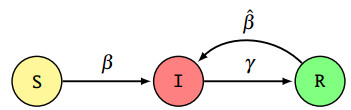
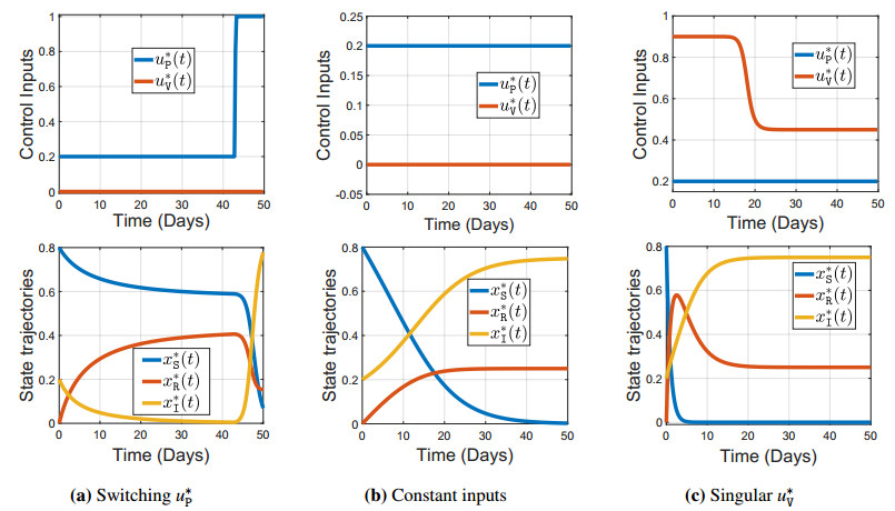
We consider the problem of the optimal allocation of vaccination and protection measures for the Susceptible-Infected-Recovered-Infected (SIRI) epidemiological model, which generalizes the classical Susceptible-Infected-Recovered (SIR) and Susceptible-Infected-Susceptible (SIS) epidemiological models by allowing for reinfection. First, we introduce the controlled SIRI dynamical model, and discuss the existence and stability of the equilibrium points. Then, we formulate a finite-horizon optimal control problem where the cost of vaccination and protection is proportional to the mass of the population that adopts it. Our main contribution in this work arises from a detailed investigation into the existence/non-existence of singular control inputs, and establishing optimality of bang-bang controls. The optimality of bang-bang control is established by solving an optimal control problem with a running cost that is linear with respect to the input variables. The input variables are associated with actions including the vaccination and imposition of protective measures (e.g., masking or isolation). In contrast to most prior works, we rigorously establish the non-existence of singular controls (i.e., the optimality of bang-bang control for our SIRI model). Under the assumption that the reinfection rate exceeds the first-time infection rate, we characterize the structure of both the optimal control inputs, and establish that the vaccination control input admits a bang-bang structure. The numerical results provide valuable insights into the evolution of the disease spread under optimal control.
- epidemics with reinfection,
- optimal control,
- switching functions,
- Lie brackets,
- bang-bang control,
- singular control
Citation: Urmee Maitra, Ashish R. Hota, Rohit Gupta, Alfred O. Hero. Optimal protection and vaccination against epidemics with reinfection risk[J]. AIMS Mathematics, 2025, 10(4): 10140-10162. doi: 10.3934/math.2025462

Related Papers:

Abstract

We consider the problem of the optimal allocation of vaccination and protection measures for the Susceptible-Infected-Recovered-Infected (SIRI) epidemiological model, which generalizes the classical Susceptible-Infected-Recovered (SIR) and Susceptible-Infected-Susceptible (SIS) epidemiological models by allowing for reinfection. First, we introduce the controlled SIRI dynamical model, and discuss the existence and stability of the equilibrium points. Then, we formulate a finite-horizon optimal control problem where the cost of vaccination and protection is proportional to the mass of the population that adopts it. Our main contribution in this work arises from a detailed investigation into the existence/non-existence of singular control inputs, and establishing optimality of bang-bang controls. The optimality of bang-bang control is established by solving an optimal control problem with a running cost that is linear with respect to the input variables. The input variables are associated with actions including the vaccination and imposition of protective measures (e.g., masking or isolation). In contrast to most prior works, we rigorously establish the non-existence of singular controls (i.e., the optimality of bang-bang control for our SIRI model). Under the assumption that the reinfection rate exceeds the first-time infection rate, we characterize the structure of both the optimal control inputs, and establish that the vaccination control input admits a bang-bang structure. The numerical results provide valuable insights into the evolution of the disease spread under optimal control.

References

[1]	C. Nowzari, V. M. Preciado, G. J. Pappas, Analysis and control of epidemics: A survey of spreading processes on complex networks, IEEE Control Syst. Mag., 36 (2016), 26–46. https://doi.org/10.1109/MCS.2015.2495000 doi: 10.1109/MCS.2015.2495000
[2]	A. Roy, C. Singh, Y. Narahari, Recent advances in modeling and control of epidemics using a mean field approach, Sādhanā, 48 (2023), 207. https://doi.org/10.1007/s12046-023-02268-z
[3]	Y. Guo, T. Li, Fractional-order modeling and optimal control of a new online game addiction model based on real data, Commun. Nonlinear Sci. Numer. Simul., 121 (2023), 107221. https://doi.org/10.1016/j.cnsns.2023.107221 doi: 10.1016/j.cnsns.2023.107221
[4]	K. H. Wickwire, Optimal isolation policies for deterministic and stochastic epidemics, Math. Biosci., 26 (1975), 325–346. https://doi.org/10.1016/0025-5564(75)90020-6 doi: 10.1016/0025-5564(75)90020-6
[5]	H. Behncke, Optimal control of deterministic epidemics, Optimal Control Appl. Methods, 21 (2000), 269–285. https://doi.org/10.1002/oca.678 doi: 10.1002/oca.678
[6]	A. Omame, N. Sene, I. Nometa, C. I. Nwakanma, E. U. Nwafor, N. O. Iheonu, et al., Analysis of COVID-19 and comorbidity co-infection model with optimal control, Optimal Control Appl. Methods, 42 (2021), 1568–1590. https://doi.org/10.1002/oca.2748 doi: 10.1002/oca.2748
[7]	D. I. Ketcheson, Optimal control of an SIR epidemic through finite-time non-pharmaceutical intervention, J. Math. Biol., 83 (2021), 7. https://doi.org/10.1007/s00285-021-01628-9 doi: 10.1007/s00285-021-01628-9
[8]	T. A. Perkins, G. España, Optimal control of the COVID-19 pandemic with non-pharmaceutical interventions, Bull. Math. Biol., 82 (2020), 118. https://doi.org/10.1007/s11538-020-00795-y doi: 10.1007/s11538-020-00795-y
[9]	T. Kruse, P. Strack, Optimal control of an epidemic through social distancing, 2020.
[10]	A. Khan, G. Zaman, Optimal control strategy of SEIR endemic model with continuous age-structure in the exposed and infectious classes, Optimal Control Appl. Methods, 39 (2018), 1716–1727. https://doi.org/10.1002/oca.2437 doi: 10.1002/oca.2437
[11]	L. Li, C. Sun, Ji. Jia, Optimal control of a delayed SIRC epidemic model with saturated incidence rate, Optimal Control Appl. Methods, 40 (2019), 367–374. https://doi.org/10.1002/oca.2482 doi: 10.1002/oca.2482
[12]	G. Gonzalez-Parra, M. Díaz-Rodríguez, A. J. Arenas, Mathematical modeling to design public health policies for Chikungunya epidemic using optimal control, Optimal Control Appl. Methods, 41 (2020), 1584–1603. https://doi.org/10.1002/oca.2621 doi: 10.1002/oca.2621
[13]	A. Omame, M. E. Isah, M. Abbas, An optimal control model for COVID-19, zika, dengue, and chikungunya co-dynamics with reinfection, Optimal Control Appl. Methods, 44 (2023), 170–204. https://doi.org/10.1002/oca.2936 doi: 10.1002/oca.2936
[14]	H. Gaff, E. Schaefer, Optimal control applied to vaccination and treatment strategies for various epidemiological models, Math. Biosci. Eng., 6 (2009), 469–492. https://doi.org/10.3934/mbe.2009.6.469 doi: 10.3934/mbe.2009.6.469
[15]	E. V. Grigorieva, E. N. Khailov, A. Korobeinikov, Optimal control for an epidemic in a population of varying size, Discret. Contin. Dyn. Syst. S, 2015 (2015), 549–561. https://doi.org/10.3934/proc.2015.0549 doi: 10.3934/proc.2015.0549
[16]	E. V. Grigorieva, E. N. Khailov, A. Korobeinikov, Optimal quarantine strategies for COVID-19 control models, Stud. Appl. Math., 147 (2021), 622–649. https://doi.org/10.1111/sapm.12393 doi: 10.1111/sapm.12393
[17]	A. Piunovskiy, A. Plakhov, M. Tumanov, Optimal impulse control of a SIR epidemic, Optimal Control Appl. Methods, 41 (2020), 448–468. https://doi.org/10.1002/oca.2552 doi: 10.1002/oca.2552
[18]	P. A. Bliman, M. Duprez, Y. Privat, N. Vauchelet, Optimal immunity control and final size minimization by social distancing for the SIR epidemic model, J. Optim. Theory Appl., 189 (2021), 408–436. https://doi.org/10.1007/s10957-021-01830-1 doi: 10.1007/s10957-021-01830-1
[19]	T. Li, Y. Guo, Modeling and optimal control of mutated COVID-19 (Delta strain) with imperfect vaccination, Chaos Solitons Fract., 121 (2023), 111825. https://doi.org/10.1016/j.chaos.2022.111825 doi: 10.1016/j.chaos.2022.111825
[20]	W. Adel, H. Gunerhan, K. S. Nisar, P. Agarwal, A. El-Mesady, Designing a novel fractional order mathematical model for COVID-19 incorporating lockdown measures, Sci. Rep., 14 (2024), 2926. https://doi.org/10.1038/s41598-023-50889-5 doi: 10.1038/s41598-023-50889-5
[21]	A. El-Mesady, A. A. Elsadany, A. M. S. Mahdy, A. Elsonbaty, Nonlinear dynamics and optimal control strategies of a novel fractional-order lumpy skin disease model, J. Comput. Sci., 79 (2024), 102286. https://doi.org/10.1016/j.jocs.2024.102286 doi: 10.1016/j.jocs.2024.102286
[22]	A. El-Mesady, H. M. Ali, The influence of prevention and isolation measures to control the infections of the fractional Chickenpox disease model, Math. Comput. Simul., 226 (2024), 606–630. https://doi.org/10.1016/j.matcom.2024.07.028 doi: 10.1016/j.matcom.2024.07.028
[23]	U. Ledzewicz, H. Schättler, On optimal singular controls for a general SIR-model with vaccination and treatment, Discrete Contin. Dyn. Syst, 2011 (2011), 981–990. https://doi.org/10.3934/proc.2011.2011.981 doi: 10.3934/proc.2011.2011.981
[24]	O. Sharomi, T. Malik, Optimal control in epidemiology, Ann. Oper. Res., 251 (2017), 55–71. https://doi.org/10.1007/s10479-015-1834-4 doi: 10.1007/s10479-015-1834-4
[25]	D. Greenhalgh, Some results on optimal control applied to epidemics, Math. Biosci., 88 (1988), 125–158. https://doi.org/10.1016/0025-5564(88)90040-5 doi: 10.1016/0025-5564(88)90040-5
[26]	R. Pagliara, B. Dey, N. E. Leonard, Bistability and resurgent epidemics in reinfection models, IEEE Control Syst. Lett., 2 (2018), 290–295. https://doi.org/10.1109/LCSYS.2018.2832063 doi: 10.1109/LCSYS.2018.2832063
[27]	I. Abouelkheir, F. El Kihal, M. Rachik, I. Elmouki, Optimal impulse vaccination approach for an SIR control model with short-term immunity, Mathematics, 7 (2019), 420. https://doi.org/10.3390/math7050420 doi: 10.3390/math7050420
[28]	T. Mapder, S. Clifford, J. Aaskov, K. Burrage, A population of bang-bang switches of defective interfering particles makes within-host dynamics of dengue virus controllable, PLoS Comput. Biol., 15 (2019), e1006668. https://doi.org/10.1371/journal.pcbi.1006668 doi: 10.1371/journal.pcbi.1006668
[29]	S. Lenhart, J. T. Workman, Optimal control applied to biological models, 1 Eds., Chapman and Hall/CRC, 2007. https://doi.org/10.1201/9781420011418
[30]	S. Y. Ren, W. B. Wang, R. D. Gao, A. M. Zhou, Omicron variant (B.1.1.529) of SARS-CoV-2: Mutation, infectivity, transmission, and vaccine resistance, World J. Clin. Cases., 10 (2022), 1–11. https://doi.org/10.12998/wjcc.v10.i1.1 doi: 10.12998/wjcc.v10.i1.1
[31]	A. Pinto, M. Aguiar, J. Martins, N. Stollenwerk, Dynamics of epidemiological models, Acta Biotheor., 58 (2010), 381–389. https://doi.org/10.1007/s10441-010-9116-7 doi: 10.1007/s10441-010-9116-7
[32]	A. Bressan, B. Piccoli, Introduction to the mathematical theory of control, 2007.
[33]	F. Blanchini, S. Miani, Set-theoretic methods in control, Birkhäuser Cham, 2015
[34]	F. Clarke, Functional analysis, calculus of variations and optimal control, London: Springer, 2013. https://doi.org/10.1007/978-1-4471-4820-3
[35]	D. Liberzon, Calculus of variations and optimal control theory: A concise introduction, Princeton University Press, 2011.
[36]	B. Bonnard, M. Chyba, Singular trajectories and their role in control theory, IEEE Trans. Automat. Control, 50 (2005), 278–279. https://doi.org/10.1109/TAC.2004.841883 doi: 10.1109/TAC.2004.841883
[37]	Q. Li, M. Med, X. Guan, P. Wu, X. Wang, Lei Zhou, et al., Early transmission dynamics in Wuhan, China, of novel coronavirus–infected pneumonia, N. Engl. J. Med., 382 (2020), 1199–1207. https://doi.org/10.1056/NEJMoa2001316 doi: 10.1056/NEJMoa2001316
[38]	Z. Du, H. Hong, S. Wang, L. Ma, C. Liu, Y. Bai, et al., Reproduction number of the Omicron variant triples that of the Delta variant, Viruses, 14 (2022), 821. https://doi.org/10.3390/v14040821 doi: 10.3390/v14040821
[39]	S. Ganguly, N. Randad, R. A. D'Silva, M. Raj, D. Chatterjee, QuITO: Numerical software for constrained nonlinear optimal control problems, SoftwareX, 24 (2023), 101557. https://doi.org/10.1016/j.softx.2023.101557 doi: 10.1016/j.softx.2023.101557
[40]	A. R. Hota, U. Maitra, E. Elokda, S. Bologonani, Learning to Mitigate epidemic risks: A dynamic population game approach, Dyn. Games Appl., 13 (2023), 1106–1129. https://doi.org/10.1007/s13235-023-00529-4 doi: 10.1007/s13235-023-00529-4

Reader Comments

Your name:*

Email:*
© 2025 the Author(s), licensee AIMS Press. This is an open access article distributed under the terms of the Creative Commons Attribution License (http://creativecommons.org/licenses/by/4.0)