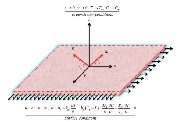
The impact of inter-particle spacing and the radius of gold nanoparticles on nanofluid flow have substantial significance across applications. Optimizing these parameters in biomedical engineering enhances the drug delivery systems, thus controlling the release of medicines and accurately targeting the targeted area. We explored nanofluid flow on a bi-directional elongated plate. The surface of the sheet was characterized with variable porosity with inclined magnetic field effects, which is the main novelty of the work. We focused on how nanoparticle radius and spacing affect the overall flow dynamics. Additionally, we incorporated the Cattaneo-Christov heat and mass flux model effects to discuss the mass and thermal diffusions using some flow conditions. The major equations were translated in dimensionless form and solved with artificial neural networks (ANNs). As outcomes, we uncovered that primary velocity has weakened with extension in stretching ratio and magnetic factors and has been amplified with progression in variable porous factor with absolute error (AE) in the range 10-3 to 10-7. Thermal panels have enlarged with escalation in thermophoresis, magnetic, radiation, and Brownian motion factors with absolute errors AEs in the range $ {10^{ - 3}} $ to $ {10^{ - 7}} $. Concentration panels have escalated with augmentation in the thermophoresis factor and activation energy factor and weakened with the expansion in Schmidt number, chemical reactivity factor, and Brownian motion factor. We conclude that the model's optimal performance has observed at epochs 111,225,194,270,179,220,339, and 221 for different scenarios. For all the scenarios, the gradient values are associated at $ 9.97 \times {10^{ - 8}} $, $ 9.91 \times {10^{ - 9}} $, $ 9.92 \times {10^{ - 8}} $, $ 9.91 \times {10^{ - 8}} $, $ 9.95 \times {10^{ - 8}} $, $ 9.91 \times {10^{ - 8}} $, $ 9.92 \times {10^{ - 8}} $, and $ 9.91 \times {10^{ - 8}} $.
Citation: Humaira Yasmin, Rawan Bossly, Fuad S. Alduais, Afrah Al-Bossly, Arshad Khan. Chemically reactive gold blood Casson nanofluid flow on a variable porous convectively heated stretching sheet with Cattaneo-Christov flux model using machine learning approach[J]. AIMS Mathematics, 2025, 10(4): 8528-8568. doi: 10.3934/math.2025392
The impact of inter-particle spacing and the radius of gold nanoparticles on nanofluid flow have substantial significance across applications. Optimizing these parameters in biomedical engineering enhances the drug delivery systems, thus controlling the release of medicines and accurately targeting the targeted area. We explored nanofluid flow on a bi-directional elongated plate. The surface of the sheet was characterized with variable porosity with inclined magnetic field effects, which is the main novelty of the work. We focused on how nanoparticle radius and spacing affect the overall flow dynamics. Additionally, we incorporated the Cattaneo-Christov heat and mass flux model effects to discuss the mass and thermal diffusions using some flow conditions. The major equations were translated in dimensionless form and solved with artificial neural networks (ANNs). As outcomes, we uncovered that primary velocity has weakened with extension in stretching ratio and magnetic factors and has been amplified with progression in variable porous factor with absolute error (AE) in the range 10-3 to 10-7. Thermal panels have enlarged with escalation in thermophoresis, magnetic, radiation, and Brownian motion factors with absolute errors AEs in the range $ {10^{ - 3}} $ to $ {10^{ - 7}} $. Concentration panels have escalated with augmentation in the thermophoresis factor and activation energy factor and weakened with the expansion in Schmidt number, chemical reactivity factor, and Brownian motion factor. We conclude that the model's optimal performance has observed at epochs 111,225,194,270,179,220,339, and 221 for different scenarios. For all the scenarios, the gradient values are associated at $ 9.97 \times {10^{ - 8}} $, $ 9.91 \times {10^{ - 9}} $, $ 9.92 \times {10^{ - 8}} $, $ 9.91 \times {10^{ - 8}} $, $ 9.95 \times {10^{ - 8}} $, $ 9.91 \times {10^{ - 8}} $, $ 9.92 \times {10^{ - 8}} $, and $ 9.91 \times {10^{ - 8}} $.

| [1] | J. B. J. Fourier, Theorie Analytique de la Chaleur, CF Didot, Paris, 1822. |
| [2] |
A. Fick, On liquid diffusion, J. Membr. Sci., 100 (1995), 33−38. https://doi.org/10.1016/0376-7388(94)00230-V doi: 10.1016/0376-7388(94)00230-V

|
| [3] | C. Cattaneo, Sulla conduzione del calore, Atti Sem. Mat. Fis. Univ. Modena, 3 (1948), 83−101. |
| [4] |
C. I. Christov, On frame indifferent formulation of the Maxwell-Cattaneo model of finite-speed heat conduction, Mech. Res. Commun., 36 (2009), 481−486. https://doi.org/10.1016/j.mechrescom.2008.11.003 doi: 10.1016/j.mechrescom.2008.11.003
|
| [5] |
M. Yaseen, S. K. Rawat, N. A. Shah, M. Kumar, S. M. Eldin, Ternary hybrid nanofluid flow containing gyrotactic microorganisms over three different geometries with Cattaneo-Christov model, Mathematics, 11 (2023), 1237. https://doi.org/10.3390/math11051237 doi: 10.3390/math11051237
|
| [6] |
S. Noreen, U. Farooq, H. Waqas, N. Fatima, M. S. Alqurashi, M. Imran, et al., Comparative study of ternary hybrid nanofluids with role of thermal radiation and Cattaneo-Christov heat flux between double rotating disks, Sci. Rep., 13 (2023), 7795. https://doi.org/10.1038/s41598-023-34783-8 doi: 10.1038/s41598-023-34783-8
|
| [7] |
M. R. Eid, M. A. El-Aziz, A. J. Alqarni, E. M. Elsaid, Numerical analysis for Cattaneo-Christov heat flux on convective viscous non-Newtonian fluid flow through porous medium with nonuniform heat source, Ain Shams Eng. J., 15 (2024), 102954. https://doi.org/10.1016/j.asej.2024.102954 doi: 10.1016/j.asej.2024.102954
|
| [8] |
M. Mumtaz, S. Islam, H. Ullah, A. Dawar, Z. Shah, A semi-analytical strategy for mixed convection non-Newtonian nanofluid flow on a stretching surface using Cattaneo-Christov model, Adv. Mech. Eng., 16 (2024), 1−13. https://doi.org/10.1177/16878132241245833 doi: 10.1177/16878132241245833
|
| [9] |
S. Rehman, Y. Trabelsi, S. Alqahtani, S. Alshehery, S. M. Eldin, A renovated Jaffrey-Hamel flow problem and new scaling statistics for heat, mass fluxes with Cattaneo-Christov heat flux model, Case Stud. Therm. Eng., 43 (2023), 1−21. https://doi.org/10.1016/j.csite.2023.102787 doi: 10.1016/j.csite.2023.102787
|
| [10] |
A. Mirzaei, P. Jalili, M. D. Afifi, B. Jalili, D. D. Ganji, Convection heat transfer of MHD fluid flow in the circular cavity with various obstacles: Finite element approach, Int. J. Thermofluids., 20 (2023), 1−14. https://doi.org/10.1016/j.ijft.2023.100522 doi: 10.1016/j.ijft.2023.100522
|
| [11] |
S. A. Lone, A. Khan, Z. Raiza, H. Alrabaiah, S. Shahab, A. Saeed, et al., A semi-analytical solution of the magnetohydrodynamic blood-based ternary hybrid nanofluid flow over a convectively heated bidirectional stretching surface under velocity slip conditions, AIP Adv., 14 (2024), 045013. https://doi.org/10.1063/5.0201663 doi: 10.1063/5.0201663
|
| [12] |
B. Ahmad, M. O. Ahmad, M. Farman, A. Akgül, M. B. Riaz, A significance of multi slip condition for inclined MHD nano-fluid flow with non linear thermal radiations, Dufuor and Sorrot, and chemically reactive bio-convection effect, S. Afr. J. Chem. Eng., 43 (2023), 135−145. https://doi.org/10.1016/j.sajce.2022.10.009 doi: 10.1016/j.sajce.2022.10.009
|
| [13] |
N. Tarakaramu, P. V. S. Narayana, N. Sivakumar, D. H. Babu, K. B. Lakshmi, Convective conditions on 3D magnetohydrodynamic (MHD) non-Newtonian nanofluid flow with nonlinear thermal radiation and heat absorption: A numerical analysis, J. Nanofluids, 12 (2023), 448−457. https://doi.org/10.1166/jon.2023.1939 doi: 10.1166/jon.2023.1939
|
| [14] |
K. Vinutha, P. Srilatha, K. Chandan, D. Sriram, J. K. Madhukesh, K. V. Nagaraja, et al., Stacking regression model approach to mixed convection flow of ternary-nanofluid over slanted surface with magnetic field, waste discharge concentration, and joule heating effects, Int. J. Thermofluids, 23 (2024), 100731. https://doi.org/10.1016/j.ijft.2024.100731 doi: 10.1016/j.ijft.2024.100731
|
| [15] |
A. M. Obalalu, M. M. Alqarni, C. Odetunde, M. A. Memon, O. A. Olayemi, A. B. Shobo, et al., Improving agricultural efficiency with solar-powered tractors and magnetohydrodynamic entropy generation in copper-silver nanofluid flow, Case Stud. Therm. Eng., 51 (2023), 103603. https://doi.org/10.1016/j.csite.2023.103603 doi: 10.1016/j.csite.2023.103603
|
| [16] |
E. A. Algehyne, F. M. Alamrani, A. Khan, K. A. Khan, S. A. Lone, A. Saeed, On thermal distribution of MHD mixed convective flow of a Casson hybrid nanofluid over an exponentially stretching surface with impact of chemical reaction and ohmic heating, Colloid Polym. Sci., 302 (2024), 503−516. https://doi.org/10.1007/s00396-023-05214-x doi: 10.1007/s00396-023-05214-x
|
| [17] | S. U. Choi, J. A. Eastman, Enhancing thermal conductivity of fluids with nanoparticles, Argonne National Lab. (ANL), Argonne, IL (United States), 1995. |
| [18] |
M. Zafar, H. Sakidin, M. Sheremet, I. B. Dzulkarnain, A. Hussain, R. Nazar, et al., Recent development and future prospective of tiwari and das mathematical model in nanofluid flow for different geometries: A review, Processes, 11 (2023), 834. https://doi.org/10.3390/pr11030834 doi: 10.3390/pr11030834
|
| [19] |
N. Anjum, W. A. Khan, M. Azam, M. Ali, M. Waqas, I. Hussain, Significance of bioconvection analysis for thermally stratified 3D Cross nanofluid flow with gyrotactic microorganisms and activation energy aspects, TSEP, 38 (2023), 101596. https://doi.org/10.1016/j.tsep.2022.101596 doi: 10.1016/j.tsep.2022.101596
|
| [20] |
D. D. Mohite, A. Goyal, A. S. Singh, M. I. Ansari, K. A. Patil, P. D. Yadav, et al., Improvement of thermal performance through nanofluids in industrial applications: A review on technical aspects, Mater. Today Proc., 2024. https://doi.org/10.1016/j.matpr.2024.04.083 doi: 10.1016/j.matpr.2024.04.083
|
| [21] |
N. Acharya, F. Mabood, S. A. Shahzad, I. A. Badruddin, Hydrothermal variations of radiative nanofluid flow by the influence of nanoparticles diameter and nanolayer, Int. Commun. Heat Mass Transf., 130 (2022). 1−15. https://doi.org/10.1016/j.icheatmasstransfer.2021.105781 doi: 10.1016/j.icheatmasstransfer.2021.105781
|
| [22] |
A. Khan, A. Saeed, A. Tassaddiq, T. Gul, S. Mukhtar, P. Kumam, et al., Bio-convective micropolar nanofluid flow over thin moving needle subject to Arrhenius activation energy, viscous dissipation and binary chemical reaction, Case Stud. Therm. Eng., 25 (2021). 1−13. https://doi.org/10.1016/j.csite.2021.100989 doi: 10.1016/j.csite.2021.100989
|
| [23] |
R. P. Gowda, R. N. Kumar, R. Kumar, B. C. Prasannakumara, Three-dimensional coupled flow and heat transfer in non-Newtonian magnetic nanofluid: An application of Cattaneo-Christov heat flux model, J. Magn. Magn. Mater., 567 (2023), 1−13. https://doi.org/10.1016/j.jmmm.2022.170329 doi: 10.1016/j.jmmm.2022.170329
|
| [24] |
H. Alrabaiah, S. Iftikhar, A. Saeed, M. Bilal, S. M. Eldin, A. M. Galal, Numerical calculation of Darcy Forchheimer radiative hybrid nanofluid flow across a curved slippery surface, S. Afr. J. Chem. Eng., 45 (2023), 172−181. https://doi.org/10.1016/j.sajce.2023.05.013 doi: 10.1016/j.sajce.2023.05.013
|
| [25] |
A. Khan, F. A. Awwad, E. A. Ismail, T. Gul, Quantitative analysis of Maxwell fluid flow with dual diffusion through the variable porous canonical gap using artificial neural network approach, Colloid Polym. Sci., 302 (2024), 1−28. https://doi.org/10.1007/s00396-024-05281-8 doi: 10.1007/s00396-024-05281-8
|
| [26] |
P. K. Yadav, S. Jaiswal, A. K. Verma, A. J. Chamkha, Magnetohydrodynamics of immiscible Newtonian fluids in porous regions of different variable permeability functions, J. Pet. Sci. Eng., 220 (2023), 1−13. https://doi.org/10.1016/j.petrol.2022.111113 doi: 10.1016/j.petrol.2022.111113
|
| [27] |
N. S. Wahid, N. M. Arifin, N. S. Khashi'ie, I. Pop, Three-dimensional unsteady radiative hybrid nanofluid flow through a porous space over a permeable shrinking surface, Chinese J. Phys., 85 (2023), 196−211. https://doi.org/10.1016/j.cjph.2023.07.016 doi: 10.1016/j.cjph.2023.07.016
|
| [28] |
M. D. Shamshuddin, G. R. Rajput, S. R. Mishra, S. O. Salawu, Radiative and exponentially space-based thermal generation effects on an inclined hydromagnetic aqueous nanofluid flow past thermal slippage saturated porous media, Int. J. Mod. Phys. B, 37 (2023), 2350202. https://doi.org/10.1142/S0217979223502028 doi: 10.1142/S0217979223502028
|
| [29] |
K. Abbas, X. H. Wang, G. Rasool, T. Sun, I. Razzaq, Thermal optimization of buoyancy driven radiative engine-oil based viscous hybrid nanofluid flow observing the micro-rotations in an inclined permeable enclosure, Case Stud. Therm. Eng., 60 (2024), 1−25. https://doi.org/10.1016/j.csite.2024.104774 doi: 10.1016/j.csite.2024.104774
|
| [30] |
P. Nagabhushana, S. Ramprasad, C. D. Prasad, H. Vasudev, C. Prakash, Numerical investigation on heat transfer of a nano-fluid saturated vertical composite porous channel packed between two fluid layers, IJIDeM, 18 (2023), 2927−2944. https://doi.org/10.1007/s12008-023-01379-5 doi: 10.1007/s12008-023-01379-5
|
| [31] |
R. Kodi, C. Ganteda, A. Dasore, M. L. Kumar, G. Laxmaiah, M. A. Hasan, et al., Influence of MHD mixed convection flow for maxwell nanofluid through a vertical cone with porous material in the existence of variable heat conductivity and diffusion, Case Stud. Therm. Eng., 44 (2023), 1−16. https://doi.org/10.1016/j.csite.2023.102875 doi: 10.1016/j.csite.2023.102875
|
| [32] |
M. Hussain, U. Farooq, M. Sheremet, Convective nanofluid flow subjected to variable porosity, inclined magnetic field, and thermal radiations, Numer. Heat Tr. B-Fund., 2023,623−640. https://doi.org/10.1080/10407790.2023.2292157 doi: 10.1080/10407790.2023.2292157
|
| [33] |
E. N. Thabet, Z. Khan, A. M. Abd-Alla, F. S. Bayones, Thermal enhancement, thermophoretic diffusion, and Brownian motion impacts on MHD micropolar nanofluid over an inclined surface: Numerical simulation, Numer. Heat Tr. A-Appl., 2023, 1−20. https://doi.org/10.1080/10407782.2023.2276319 doi: 10.1080/10407782.2023.2276319
|
| [34] |
K. R. Madhura, Babitha, Numerical study on magnetohydrodynamics micropolar Carreau nanofluid with Brownian motion and thermophoresis effect, Int. J. Model. Simul., 45 (2023), 651−664. https://doi.org/10.1080/02286203.2023.2234240 doi: 10.1080/02286203.2023.2234240
|
| [35] |
H. A. Madkhali, M. Ahmed, M. Nawaz, S. O. Alharbi, A. S. Alqahtani, M. Y. Malik, Computational study on the effects of Brownian motion and thermophoresis on thermal performance of cross fluid with nanoparticles in the presence of Ohmic and viscous dissipation in chemically reacting regime, Comput. Part. Mech., 11 (2024), 1301−1311. https://doi.org/10.1007/s40571-023-00687-7 doi: 10.1007/s40571-023-00687-7
|
| [36] |
N. Sandeep, P. Nanda, C. Sulochana, G. P. Ashwinkumar, Dynamics of Casson/Carreau hybrid nanofluid flow over a wedge with thermophoresis and Brownian motion effects, Int. J. Model. Simul., 2024, 1−12. https://doi.org/10.1080/02286203.2024.2345245 doi: 10.1080/02286203.2024.2345245
|
| [37] |
H. Waqas, S. A. Khan, B. Ali, D. Liu, T. Muhammad, E. Hou, Numerical computation of Brownian motion and thermophoresis effects on rotational micropolar nanomaterials with activation energy, Propuls. Power Res., 12 (2023), 397−409. https://doi.org/10.1016/j.jppr.2023.05.005 doi: 10.1016/j.jppr.2023.05.005
|
| [38] |
B. K. Sharma, U. Khanduri, N. K. Mishra, K. S. Mekheimer, Combined effect of thermophoresis and Brownian motion on MHD mixed convective flow over an inclined stretching surface with radiation and chemical reaction, Int. J. Mod. Phys. B, 37 (2023), 2350095. https://doi.org/10.1142/S0217979223500959 doi: 10.1142/S0217979223500959
|
| [39] |
R. R. Vaddemani, S. Ganta, R. Kodi, Effects of hall current, activation energy and diffusion thermo of MHD Darcy-Forchheimer Casson nanofluid flow in the presence of Brownian motion and thermophoresis, J. Adv. Res. Fluid Mech. Therm. Sci., 105 (2023), 129−145. https://doi.org/10.37934/arfmts.105.2.129145 doi: 10.37934/arfmts.105.2.129145
|
| [40] |
F. Almeida, B. J. Gireesha, P. Venkatesh, Magnetohydrodynamic flow of a micropolar nanofluid in association with Brownian motion and thermophoresis: Irreversibility analysis, Heat Trans., 52 (2023), 2032−2055. https://doi.org/10.1002/htj.22773 doi: 10.1002/htj.22773
|
| [41] |
T. P. Kumar, G. Dharmaiah, K. Al-Farhany, A. Abdulkadhim, M. A. Alomari, M. H. Abdulsada, et al., Transient conditions effects on electromagnetic casson fluid flow via stretching surface: System thermal case elaboration, Numer. Heat Tr. B-Fund., 84 (2023), 539−555. https://doi.org/10.1080/10407790.2023.2215406 doi: 10.1080/10407790.2023.2215406
|
| [42] |
M. R. Islam, S. Reza‐E‐Rabbi, M. Y. Ali, M. M. H. Rasel, S. F. Ahmmed, Numerical simulation of mass and heat transport phenomena of hydromagnetic flow of Casson fluid with sinusoidal boundary conditions, Eng Rep., 5 (2023), e12659. https://doi.org/10.1002/eng2.12659 doi: 10.1002/eng2.12659
|
| [43] |
Z. Mahmood, M. Ur Rehman, U. Khan, B. Ali, M. I. H. Siddiqui, Enhanced transport phenomena in Casson fluid flow over radiative moving surface: Influence of velocity and thermal slip conditions with mixed convection and chemical reaction, Mod. Phys. Lett. B, 39 (2024), 2450383. https://doi.org/10.1142/S0217984924503834 doi: 10.1142/S0217984924503834
|
| [44] |
H. Upreti, S. R. Mishra, A. K. Pandey, N. Joshi, B. P. Joshi, Diversified role of fuzzified particle concentration on Casson gold-blood nanofluid flow through an elongating sheet for different shape nanoparticles, J. Taibah Univ. Sci., 17 (2023), 2254465. https://doi.org/10.1080/16583655.2023.2254465 doi: 10.1080/16583655.2023.2254465
|
| [45] |
N. M. Hafez, A. M. Abd-Alla, T. M. N. Metwaly, Influences of rotation and mass and heat transfer on MHD peristaltic transport of Casson fluid through inclined plane, Alex. Eng. J., 68 (2023), 665−692. https://doi.org/10.1016/j.aej.2023.01.038 doi: 10.1016/j.aej.2023.01.038
|
| [46] |
M. Hussain, U. Farooq, M. Sheremet, Nonsimilar convective thermal transport analysis of EMHD stagnation Casson nanofluid flow subjected to particle shape factor and thermal radiations, Int. Commun. Heat Mass Transf., 137 (2022), 106230. https://doi.org/10.1016/j.icheatmasstransfer.2022.106230 doi: 10.1016/j.icheatmasstransfer.2022.106230
|
| [47] |
H. Yasmin, H. A. Hejazi, S. A. Lone, Z. Raizah, A. Saeed, Time-independent three-dimensional flow of a water-based hybrid nanofluid past a Riga plate with slips and convective conditions: A homotopic solution, Nanotechnol. Rev., 12 (2023), 1−13. https://doi.org/10.1515/ntrev-2023-0183 doi: 10.1515/ntrev-2023-0183
|
| [48] |
A. Dawar, S. Islam, Z. Shah, S. R. Mahmuod, S. A. Lone, Dynamics of inter-particle spacing, nanoparticle radius, inclined magnetic field and nonlinear thermal radiation on the water-based copper nanofluid flow past a convectively heated stretching surface with mass flux condition: A strong suction case, Int. Commun. Heat Mass Transf., 137 (2022), 106286. https://doi.org/10.1016/j.icheatmasstransfer.2022.106286 doi: 10.1016/j.icheatmasstransfer.2022.106286
|
| [49] |
T. A. Yusuf, F. Mabood, W. A. Khan, J. A. Gbadeyan, Irreversibility analysis of Cu-TiO2-H2O hybrid-nanofluid impinging on a 3-D stretching sheet in a porous medium with nonlinear radiation: Darcy-Forchhiemer's model, Alex. Eng. J., 59 (2020), 5247−5261. https://doi.org/10.1016/j.aej.2020.09.053 doi: 10.1016/j.aej.2020.09.053
|
| [50] |
S. Srinivas, A. Vijayalakshmi, A. S. Reddy, Flow and heat transfer of gold-blood nanofluid in a porous channel with moving/stationary walls, J. Mech., 33 (2017), 395−404. https://doi.org/10.1017/jmech.2016.102 doi: 10.1017/jmech.2016.102
|
| [51] |
R. S. Reddy Gorla, I. Sidawi, Free convection on a vertical stretching surface with suction and blowing, Appl. Sci. Res., 52 (1994), 247−257. https://doi.org/10.1007/BF00853952 doi: 10.1007/BF00853952
|
| [52] |
M. A. A. Hamad, Analytical solution of natural convection flow of a nanofluid over a linearly stretching sheet in the presence of magnetic field, Int. Commun. Heat Mass Transf., 38 (2011), 487−492. https://doi.org/10.1016/j.icheatmasstransfer.2010.12.042 doi: 10.1016/j.icheatmasstransfer.2010.12.042
|


Figures(24) / Tables(3)

Humaira Yasmin, Rawan Bossly, Fuad S. Alduais, Afrah Al-Bossly, Arshad Khan. Chemically reactive gold blood Casson nanofluid flow on a variable porous convectively heated stretching sheet with Cattaneo-Christov flux model using machine learning approach[J]. AIMS Mathematics, 2025, 10(4): 8528-8568. doi: 10.3934/math.2025392


 DownLoad: