Two parameter log-Lindley distribution with LTPL web-tool

Emrah Altun; Christophe Chesneau; Hana N. Alqifari; Emrah Altun; Christophe Chesneau; Hana N. Alqifari

doi:10.3934/math.2025382

AIMS Mathematics

2025, Volume 10, Issue 4: 8306-8321. doi: 10.3934/math.2025382

Previous Article Next Article

Research article Special Issues

Two parameter log-Lindley distribution with LTPL web-tool

1.
Department of Mathematics, Bartin University, Bartin 74100, Turkey
2.
Department of Mathematics, University of Caen-Normandie, Caen 14000, France
3.
Department of Statistics and Operations Research, College of Science, Qassim University, Saudi Arabia

Received: 02 December 2024 Revised: 21 February 2025 Accepted: 21 March 2025 Published: 11 April 2025
MSC : 62E15

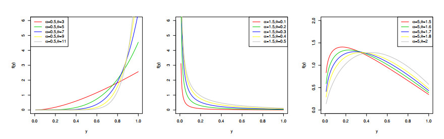
This paper introduces the two-parameter log-Lindley distribution. It can be presented as a new flexible distribution supported on the interval $(0, 1)$ , which includes the famous log-Lindley distribution as a sub-distribution. Its important probabilistic properties are discussed. On the applied side, a statistical focus was placed on the corresponding model. Three methods were used for the parameter estimation and the effectiveness of these methods was evaluated by a simulation study. The superiority of the proposed distribution over other distributions was demonstrated with three applications on real data sets. A significant aspect of the study is the development of an associated web tool. The LTPL web tool was designed to enable users to utilize the newly developed probability distribution without requiring any programming expertise.

Keywords:

Citation: Emrah Altun, Christophe Chesneau, Hana N. Alqifari. Two parameter log-Lindley distribution with LTPL web-tool[J]. AIMS Mathematics, 2025, 10(4): 8306-8321. doi: 10.3934/math.2025382

Related Papers:

[1]	M. R. Irshad, S. Aswathy, R. Maya, Amer I. Al-Omari, Ghadah Alomani . A flexible model for bounded data with bathtub shaped hazard rate function and applications. AIMS Mathematics, 2024, 9(9): 24810-24831. doi: 10.3934/math.20241208
[2]	Ahmed M. Gemeay, Najwan Alsadat, Christophe Chesneau, Mohammed Elgarhy . Power unit inverse Lindley distribution with different measures of uncertainty, estimation and applications. AIMS Mathematics, 2024, 9(8): 20976-21024. doi: 10.3934/math.20241021
[3]	Doaa Basalamah, Bader Alruwaili . The weighted Lindley exponential distribution and its related properties. AIMS Mathematics, 2023, 8(10): 24984-24998. doi: 10.3934/math.20231275
[4]	Emrah Altun, Mustafa Ç. Korkmaz, M. El-Morshedy, M. S. Eliwa . The extended gamma distribution with regression model and applications. AIMS Mathematics, 2021, 6(3): 2418-2439. doi: 10.3934/math.2021147
[5]	SidAhmed Benchiha, Amer Ibrahim Al-Omari, Naif Alotaibi, Mansour Shrahili . Weighted generalized Quasi Lindley distribution: Different methods of estimation, applications for Covid-19 and engineering data. AIMS Mathematics, 2021, 6(11): 11850-11878. doi: 10.3934/math.2021688
[6]	Emrah Altun, Hana Alqifari, Mohamed S. Eliwa . A novel approach for zero-inflated count regression model: Zero-inflated Poisson generalized-Lindley linear model with applications. AIMS Mathematics, 2023, 8(10): 23272-23290. doi: 10.3934/math.20231183
[7]	Fiaz Ahmad Bhatti, Azeem Ali, G. G. Hamedani, Mustafa Ç. Korkmaz, Munir Ahmad . The unit generalized log Burr XII distribution: properties and application. AIMS Mathematics, 2021, 6(9): 10222-10252. doi: 10.3934/math.2021592
[8]	Haiping Ren, Xue Hu . Estimation for inverse Weibull distribution under progressive type-Ⅱ censoring scheme. AIMS Mathematics, 2023, 8(10): 22808-22829. doi: 10.3934/math.20231162
[9]	Vladica S. Stojanović, Hassan S. Bakouch, Radica Bojičić, Gadir Alomair, Shuhrah A. Alghamdi . Poisson-Lindley minification INAR process with application to financial data. AIMS Mathematics, 2024, 9(8): 22627-22654. doi: 10.3934/math.20241102
[10]	Aliyu Ismail Ishaq, Abdullahi Ubale Usman, Hana N. Alqifari, Amani Almohaimeed, Hanita Daud, Sani Isah Abba, Ahmad Abubakar Suleiman . A new Log-Lomax distribution, properties, stock price, and heart attack predictions using machine learning techniques. AIMS Mathematics, 2025, 10(5): 12761-12807. doi: 10.3934/math.2025575

Abstract

1. Introduction

The distributions supported on the unit interval, i.e., $(0, 1)$ , are used in a variety of fields, including engineering, economics, and biology. Their importance has increased in recent literature, which explores innovative modeling approaches through techniques such as random variable transformation, function composition, and the development of new families of distributions. The most popular transformation remains the exponential transformation, which deals with random variables of the form $Y=\exp\left(-X\right)$ , where $X$ denotes a random variable with a certain lifetime distribution, i.e., supported on $(0, +\infty)$ . Using this transformation, the log-WE distribution by ^[2], the log-xgamma distribution by ^[4], the log-ISDL distribution by ^[3], and the unit Weibull distribution by ^[35] were proposed. More recently, ^[24] introduced the log-cosine power distribution and compared its performance with several competing distributions also defined on $(0, 1)$ . ^[8] developed a new unit power distribution using the Gamma/Gompertz distribution as the baseline distribution. ^[15] contributed to the topic by proposing a version of the log-log distribution supported on $(0, 1)$ , called the unit log-log distribution. ^[27] defined a new unit distribution using $Y=X_1 / \left(X_1+ X_2\right)$ , where $X_1$ and $X_2$ are two independent random variables with Weibull distributions having the same shape parameter and scale parameter equal to 1. ^[6] proposed another useful distribution based on $Y=X/\left(X+1\right)$ , where $X$ is a random variable with the Zeghdoudi distribution. ^[12] used the truncation approach on the Chris-Jerry distribution to obtain a distribution supported on the unit interval. ^[26] applied $Y=\exp\left(-X\right)$ , where $X$ is a random variable with the half-logistic-geometric distribution, proposed by ^[21].

In terms of statistical applications, the beta regression model is the first option that comes to mind to model a dependent variable defined in the range $(0, 1)$ . However, newly defined distributions supported on $(0, 1)$ have allowed the definition of different regression models that prove to be quite competitive. More specifically, new regression models have been proposed using mean-parameterized versions of distributions that are more flexible than the beta distribution. Thus, different modeling methods have been developed with successful applications. Among them, ^[23] defined the unit-Lindley distribution based on $Y=X/\left(X+1\right)$ , where $X$ is a random variable with the Lindley distribution, and introduced the unit-Lindley regression model. This model attracted considerable interest from researchers. Using the same idea, many regression models have been proposed, such as the unit Burr-XII regression model by ^[17], the unit Chen regression model by ^[18], the log-Bilal regression model by ^[5], and the log-exponential power regression model by ^[19].

Among the developments in lifetime distributions, ^[29] proposed a new generalization of the Lindley distribution by adding a scale parameter. This distribution is called the two-parameter Lindley (TPL) distribution. It is defined with the probability density function (pdf) given by

$\begin{equation} f\left( {x;\alpha , \theta } \right) = \frac{{{\theta ^2}}}{{\theta + \alpha }}\left( {1 + \alpha x} \right)\exp \left( { - \theta x} \right), \end{equation}$

(1.1)

where $x>0$ and $\alpha, \theta>0$ are both scale parameters. One of the important properties of the TPL distribution is that, when $\alpha=1$ , it becomes the Lindley distribution. The TPL distribution is also equivalent to the exponential distribution for $\alpha=0$ . With these remarkable properties in mind, and the idea of innovating in the field of statistical modeling with data in the range $(0, 1)$ , we come up with the idea described below. Using the exponential transformation $Y=\exp\left(-X\right)$ , where $X$ is a random variable with the TPL distribution, $Y$ follows a new distribution support on $(0, 1)$ , which we call the log-TPL (LTPL) distribution. To the best of our knowledge, it offers a new statistical perspective. Among its notable properties, the LTPL distribution includes the log-Lindley and log-exponential distributions as its sub-distributions. Although numerous distributions have been proposed by researchers, there is still a lack of software support to facilitate the practical application of the corresponding model. In response to this gap, we are developing the LTPL cloud-based web-tool to improve the accessibility and usability of the LTPL model.

The remaining sections of the study are organized as follows: Section 2 focuses on the properties of the LTPL distribution. Section 3 demonstrates three applications of the corresponding LTPL model using real data sets. Section 4 introduces the LTPL web-tool. Section 5 concludes the study.

2. LTPL distribution

This section discusses the mathematical and statistical foundations of the LTPL distribution described above.

2.1. Important properties

First, let $X$ be a random variable with TPL distribution and $Y=\exp\left(-X\right)$ . Then the pdf of $Y$ is given by

$\begin{equation*} f\left( {y;\alpha , \theta } \right) = \frac{{{\theta ^2}{y^{\theta - 1}}\left( {1 - \alpha \log \left( y \right)} \right)}}{{\alpha + \theta }}, \end{equation*}$

where $0 < y < 1$ , $\theta>0$ is the shape, and $\alpha>0$ is the scale parameter. In the remaining sections of the study, the resulting distribution is denoted as $\text{LTPL}(\alpha, \theta)$ . Given the above framework, the cumulative distribution function (cdf) of the LTPL distribution is

$\begin{equation*} F\left( {y;\alpha , \theta } \right) = \frac{{{y^\theta }\left( {\alpha + \theta - \alpha \theta \log \left( y \right)} \right)}}{{\alpha + \theta }}, \end{equation*}$

and its survival function (sf) is

$\begin{equation*} S\left( {y;\alpha , \theta } \right) = \frac{{ {(\alpha + \theta)(1-y^\theta) +\alpha \theta y^\theta }\log \left( y \right)} }{{\alpha + \theta }}. \end{equation*}$

In addition, the hazard rate function (hrf) is

$\begin{equation*} h\left( {y;\alpha , \theta } \right) = \frac{{{\theta ^2}\left( {1 - \alpha \log \left( y \right)} \right)}}{{y\left( {\alpha \theta \log \left( y \right) - \left( {\alpha + \theta } \right){y^{ - \theta }}\left( {{y^{ - \theta }} - 1} \right)} \right)}}. \end{equation*}$

These functions are central to the LTPL distribution and will be discussed later under a special configuration of the parameters depending on the mean of $Y$ . In this context, for any positive integer $r$ the raw moments of order $r$ of the LTPL distribution can be obtained by the following integral development:

$\begin{align*} E\left( {{Y^r}} \right) &= \int_0^1y^r f\left( {y;\alpha , \theta } \right)dy = \int_0^1 {{y^r}\frac{{{\theta ^2}{y^{\theta - 1}}\left( {1 - \alpha \log \left( y \right)} \right)}}{{\alpha + \theta }}} dy \nonumber\\ &= \frac{\theta^2}{\alpha+\theta} \int_0^1y^{r+\theta-1} dy-\frac{\theta^2 \alpha}{\alpha+\theta} \int_0^1y^{r+\theta-1} \log \left( y \right)dy \nonumber\\ & = \frac{\theta^2}{\alpha+\theta}\times \frac{1}{r+\theta}-\frac{\theta^2 \alpha}{\alpha+\theta}\times \left[-\frac{1}{(r+\theta)^2}\right] \nonumber \\ & = \frac{{{\theta ^2}\left( {\alpha + \theta + r} \right)}}{{\left( {\alpha + \theta } \right){{\left( {\theta + r} \right)}^2}}}. \end{align*}$

For $r=1$ , we have the mean of the LTPL distribution, given by

$\begin{equation} \mu= E\left( Y \right) = \frac{{{\theta ^2}\left( {\alpha + \theta + 1} \right)}}{{\left( {\alpha + \theta } \right){{\left( {\theta + 1} \right)}^2}}}. \end{equation}$

(2.1)

Using Eq (2.1), the mean-parametrized LTPL distribution can be obtained. Using the following transformation:

$\begin{equation*} \alpha = \frac{{\theta \left( {\theta + 1} \right)\left[ {\theta \left( {\mu - 1} \right) + \mu } \right]}}{{{\theta ^2}\left( {1 - \mu } \right) - 2\theta \mu - \mu }}, \end{equation*}$

we get

$\begin{equation} f\left( {y;\mu , \theta } \right) = \frac{{{\theta ^2}{y^{\theta - 1}}\left\lbrace {1 - \theta \left( {\theta + 1} \right)\left[ {\theta \left( {\mu - 1} \right) + \mu } \right]{{\left[ {{\theta ^2}\left( {1 - \mu } \right) - 2\theta \mu - \mu } \right]}^{ - 1}}\log \left( y \right)} \right\rbrace}}{{\theta \left( {\theta + 1} \right)\left[ {\theta \left( {\mu - 1} \right) + \mu } \right]{{\left[ {{\theta ^2}\left( {1 - \mu } \right) - 2\theta \mu - \mu } \right]}^{ - 1}} + \theta }}, \end{equation}$

(2.2)

where $0 <y<1$ and $\theta>0$ is the scale parameter. We mention that $0<\mu<1$ , which is an essential condition. In the following, the distribution defined by the pdf in Eq (2.2) is referred to as $\text{LTPL}\left(\mu, \alpha\right)$ . The pdf shapes for different parameter values are shown in Figure 1. Accordingly, the proposed distribution can take right-skewed and left-skewed shapes. It is expected to give successful results in modeling extremely right-skewed or left-skewed data.

Figure 1. Pdf plots.

DownLoad: Full-Size Img PowerPoint

The pdf shapes based on the different parameter value regions are displayed in Figure 2. The nature of these regions confirm the shapes of the LTPL distribution displayed in Figure 1, i.e., the LTPL distribution has three different shapes: increasing, decreasing, and increasing-decreasing.

Figure 2. Pdf regions.

DownLoad: Full-Size Img PowerPoint

The mean and variance values of the LTPL distribution are shown in . When the results of this figure are analyzed in detail, the following conclusions can be drawn. The mean of the LTPL distribution is an increasing function of $\theta$ and a decreasing function of $\alpha$ . However, when the variance values are examined, it is an increasing-decreasing function of $\theta$ and a decreasing function of $\alpha$ .

Figure 3. Mean and variance plots.

DownLoad: Full-Size Img PowerPoint

The shapes of the hrf of the LTPL distribution are studied according to different parameter values and the results are shown in Figure 4. As can be seen, the LTPL distribution has two different hazard shapes as increasing and bathtub. Distributions with such different hazard shapes are very important in reliability and lifetime modeling.

Figure 4. Hrf regions.

DownLoad: Full-Size Img PowerPoint

To verify the results in Figure 4, we also plot the possible shapes of the hrf using different parameter values in Figure 5. It can clearly be seen that the results obtained in Figures 4 and 5 confirm each other. The LTPL distribution has some limitations. In particular, it cannot be used for analyzing bimodal data sets. It is also evident that it is not sufficiently successful in analyzing data with a decreasing hrf structure.

Figure 5. Hrf plots.

DownLoad: Full-Size Img PowerPoint

The LTPL distribution contains two notable distributions as its sub-distributions.

$\checkmark$ When $\alpha=1$ , the LTPL distribution reduces to the log-Lindley distribution.

$\checkmark$ When $\alpha=0$ , the LTPL distribution reduces to the log-exponential distribution.

We conclude this subsection with some interesting theoretical material on the LTPL distribution, omitting the details for the sake of brevity.

The Lorenz curve of the LTPL distribution is given by

$\begin{equation*} L\left( {t;\alpha , \theta } \right) = \frac{{{t^{\theta + 1}}\left( {\alpha + \theta - \alpha \log \left( t \right) - \alpha \theta \log \left( t \right) + 1} \right)}}{{\alpha + \theta + 1}}, \end{equation*}$

where $0 < t < 1$ .

Using similar arguments that those in Eq (2.1), the incomplete moment of the LTPL distribution is obtained as

$\begin{equation*} m\left( {t;\alpha , \theta } \right) = \frac{{{t^{\theta + 1}}{\theta ^2}\left( {\alpha + \theta - \alpha \log \left( t \right) - \alpha \theta \log \left( t \right) + 1} \right)}}{{\left( {\alpha + \theta } \right){{\left( {\theta + 1} \right)}^2}}}, \end{equation*}$

where $0 < t < 1$ .

The inverse-transform method can be used to generate random observations from the LTPL distribution. However, this method requires the expression of the corresponding quantile function to be obtained. Since the solution of the equation $F\left({y;\alpha, \theta } \right) =u$ for $y$ cannot be obtained in closed form (or with the use of the Lambert function, which remains a special function), the quantile function is not easily manipulable. In this case, random observations from the LTPL distribution can be generated using the non-linear equation solver.

2.2. Estimation

Let us now discuss the parameter estimation of the LTPL model derived from the LTPL distribution. Let $Y$ be a random variable with the LTPL distribution, $n$ be a positive integer, and $y_1, \ldots, y_n$ be independent observations of $Y$ , representing the data. In this framework, the log-likelihood function of the LTPL distribution is

$\begin{equation} \ell \left( {\alpha , \theta } \right) = 2n\log \left( \theta \right) + \left( {\theta - 1} \right)\sum\limits_{i = 1}^n {\log \left( {{y_i}} \right) + } \sum\limits_{i = 1}^n {\log \left( {1 - \alpha \log \left( {{y_i}} \right)} \right)} - n\log \left( {\alpha + \theta } \right). \end{equation}$

(2.3)

If we differentiate the function in Eq (2.3) according to the parameters, we obtain

$\begin{equation} \frac{{\partial \ell \left( {\alpha , \theta } \right)}}{{\partial \alpha }} = \sum\limits_{i = 1}^n {\frac{{\log \left( {{y_i}} \right)}}{{1 - \alpha \log \left( {{y_i}} \right)}}} - n\frac{1}{{\alpha + \theta }} \end{equation}$

(2.4)

and

$\begin{equation} \frac{{\partial \ell \left( {\alpha , \theta } \right)}}{{\partial \theta }} = 2n\frac{1}{\theta } + \sum\limits_{i = 1}^n {\log \left( {{y_i}} \right) } - n\frac{1}{{\alpha + \theta }}. \end{equation}$

(2.5)

The simultaneous solution of ${{\partial \ell \left({\alpha, \theta } \right)}}/({{\partial \alpha }})=0$ and ${{\partial \ell \left({\alpha, \theta } \right)}}/({{\partial \theta }})=0$ according to $\alpha$ and $\theta$ based on Eqs (2.4) and (2.5) gives the maximum likelihood (ML) estimates of $\alpha$ and $\theta$ . However, as is obvious, there are no explicit solutions for these equations. Therefore, the log-likelihood function in Eq (2.3) has to be maximized using optimization algorithms. For this purpose, we use the optim function of the R software with the Nelder-Mead algorithm. The observed information matrix (OIM) is used to obtain the asymptotic standard errors of the estimated parameters. The components of the OIM are

$\begin{equation} {I_{\alpha \alpha }} = \sum\limits_{i = 1}^n {\frac{{\log {{\left( {{y_i}} \right)}^2}}}{{{{\left( {1 - \alpha \log \left( {{y_i}} \right)} \right)}^2}}}} + \frac{n}{{{{\left( {\alpha + \theta } \right)}^2}}}, \end{equation}$

(2.6)

$\begin{equation} {I_{\alpha \theta }} = \frac{n}{{{{\left( {\alpha + \theta } \right)}^2}}}, \end{equation}$

(2.7)

and

$\begin{equation} {I_{\theta \theta }} = n\left( {\frac{1}{{{{\left( {\alpha + \theta } \right)}^2}}} - \frac{2}{{{\theta ^2}}}} \right). \end{equation}$

(2.8)

The OIM, evaluated at $\hat{\alpha}$ and $\hat{\theta}$ , is automatically calculated in the optim function. In addition to the MLE, the parameters of the LTPL distribution can be estimated with different methods, namely least squares (LS) and weighted LS (WLS) estimation methods. They consist in minimizing the difference between the empirical and theoretical distribution functions. For a more detailed description, let $y_{1:n}, \ldots, y_{n:n}$ be the ordered observations of $Y$ . The objective function of the LS method for the LTPL distribution is

$\begin{equation} \sum\limits_{i = 1}^n {{{\left[ {\frac{{y_{i:n}^\theta \left( {\alpha + \theta - \alpha \theta \log \left( {{y_{i:n}}} \right)} \right)}}{{\alpha + \theta }} - \frac{i}{{n + 1}}} \right]}^2}}. \end{equation}$

(2.9)

The WLS method is used when the observations have varying variance. The associated objective function is

$\begin{equation} \sum\limits_{i = 1}^n {\frac{{{{\left( {n + 1} \right)}^2}\left( {n + 2} \right)}}{{i\left( {n - i + 1} \right)}}{{\left[ {\frac{{y_{i:n}^\theta \left( {\alpha + \theta - \alpha \theta \log \left( {{y_{i:n}}} \right)} \right)}}{{\alpha + \theta }} - \frac{i}{{n + 1}}} \right]}^2}}. \end{equation}$

(2.10)

The objective functions in Eqs (2.9) and (2.10) are minimized using the optim function that is located in the R software.

2.3. Simulation

The simulation study is used to compare the effectiveness of the three different parameter estimation methods presented in the previous section. The number of simulation replications is set to 1000. The parameters of the LTPL distribution are chosen as $\alpha=0.5$ and $\theta=0.5$ . The results obtained are summarized in Table 1. They are evaluated according to the bias, mean square error (MSE), and mean relative error (MRE) results. The findings are briefly presented as follows.

Table 1. Simulation results.

Sample sizes	Metrics	LSE		WLSE		MLE
Sample sizes	Metrics	$\alpha$	$\theta$	$\alpha$	$\theta$	$\alpha$	$\theta$
100	Bias	0.4543	0.0420	0.2790	0.0330	0.1807	-0.0108
	MSE	0.7958	0.0054	0.5797	0.0048	0.5628	0.0080
	MRE	1.9086	1.0839	1.5580	1.0829	1.3613	0.9784
300	Bias	0.2547	0.0361	0.2127	0.0282	0.0546	-0.0049
	MSE	0.1659	0.0025	0.1506	0.0020	0.1294	0.0030
	MRE	1.5093	1.0723	1.4254	1.0664	1.1092	0.9903
500	Bias	0.2300	0.0345	0.2069	0.0150	0.0342	-0.0027
	MSE	0.1105	0.0019	0.1074	0.0017	0.0589	0.0015
	MRE	1.4600	1.0689	1.3538	1.0557	1.0683	0.9946
1000	Bias	0.2181	0.0348	0.2630	0.0401	0.0264	-0.0004
	MSE	0.0721	0.0015	0.0966	0.0019	0.0275	0.0007
	MRE	1.4363	1.0696	1.3261	1.0402	1.0529	0.9992

| Show Table

DownLoad: CSV

$\checkmark$ It can clearly be seen that the bias and MSE values approach 0 as the sample size increases. However, the MLE method was the fastest method to approach 0.

$\checkmark$ Similarly, the MRE values for all three parameter estimation methods were found to approach the value of 1 for sufficiently large samples.

$\checkmark$ The results show that all three methods provide asymptotically unbiased estimates. However, as the MLE method was found to give better results for small samples, it is more appropriate to use it for statistical purposes based on the LTPL distribution.

3. Applications

3.1. Failure time

^[24] introduced the log-cosine-power (LCP) distribution and tested its performance on the data set about the failure times of Kevlar 49/epoxy strands tested at a 90% stress level. The data set can be found in ^[24] and ^[30]. Furthermore, ^[24] compared the LCP distribution with the following distributions: the unit Teissier distribution by ^[20], the transmuted unit Rayleigh distribution by ^[16], the Topp-Leone distribution by ^[32], the unit exponential distribution by ^[7], and the unit Burr XII distribution by ^[28].

We use the same data set and standard criteria, i.e., AIC, AICc, BIC, KS, and the p-value of the KS test, to demonstrate the flexibility of the LTPL distribution across these competitive models. The results obtained are shown in Table 2. As the results of these competing models are given in ^[24], they are omitted. The LTPL distribution has the lowest goodness-of-fit statistics and the highest p-value for the KS test. Thus, it has a better modeling ability than the other six distributions.

Table 2. Results of the LTPL distribution for failure times data.

Parameters	Estimates	Std. Errors	$-\ell$	AIC	AICc	BIC	KS	p-value
$\theta$	0.899	0.193	5.988	7.976	7.758	3.855	0.098	0.634
$\alpha$	0.498	0.648

| Show Table

DownLoad: CSV

The total time of test (TTT) plot ^[1] in Figure 6 shows that the data set has a bathtub hazard shape. Therefore, it can be efficiently analyzed by the LTPL distribution. The corresponding fitted functions, namely the fitted pdf, hrf, and sf, supplemented by a probability-probability (PP) plot, are also displayed in Figure 6. These plots show that the LTPL distribution is a good choice for the data.

Figure 6. Graphical results of the LTPL distribution for failure time data and the TTT plot.

DownLoad: Full-Size Img PowerPoint

3.2. French speakers

The data set is about the geographical distribution of French speakers for 88 countries. It was collected in 2014 and can be found in ^[13]. ^[13] analyzed the data using the beta distribution, the Kumaraswamy distribution, the log-Lindley distribution introduced by ^[11], the transformed Leipnik distribution by ^[14], and the two-sided power distribution by ^[33].

Table 3 contains the estimated parameters of the LTPL distribution for these data. We compare it with the distributions used in ^[13]. The LTPL distribution has the lowest values of the model selection criteria. Therefore, it gives better results than other competing distributions.

Table 3. Results of the LTPL distribution for French speakers data.

Parameters	Estimates	Std. Errors	$-\ell$	AIC	AICc	BIC	KS	p-value
$\theta$	6.280	5.981	-56.894	-109.788	-109.646	-104.833	0.073	0.734
$\alpha$	0.775	0.069

| Show Table

DownLoad: CSV

As displayed in Figure 7, the data set has a bathtub hazard shape which can be easily modeled by the LTPL distribution. In addition, the fitted pdf and PP plot of the LTPL distribution confirm its good modeling performance.

Figure 7. Graphical results of the LTPL distribution for French speakers data and the TTT plot.

DownLoad: Full-Size Img PowerPoint

3.3. Antimicrobial resistance

This data set was concerned with the antimicrobial resistance of 24 individuals and was used by ^[25] and fitted to the unit Omega distribution. We also use the same data set for the LTPL distribution and the results are given in Table 4. The LTPL distribution has lower goodness-of-fit statistics than the beta and Kumaraswamy distributions. The results of the competition models are available in the study by ^[25]. Figure 8 shows the accuracy of the LTPL distribution in representing the data of interest.

Table 4. Results of the LTPL distribution for antimicrobial resistance data.

Parameters	Estimates	Std. Errors	$-\ell$	AIC	AICc	BIC	KS	p-value
$\theta$	15.866	38.010	-7.871	-11.743	-11.171	-9.387	0.104	0.956
$\alpha$	1.092	0.176

| Show Table

DownLoad: CSV

Figure 8. Graphical results of the LTPL distribution for antimicrobial resistance data and the TTT plot.

DownLoad: Full-Size Img PowerPoint

4. LTPL: Shiny web-tool

As highlighted in the previous sections, a variety of unit distributions have been proposed by researchers. However, their practical use is often limited for practitioners who do not have programming expertise in R or Python. To overcome this limitation in our study, we have developed a web-based tool that aims to make the LTPL distribution more accessible and practical. The LTPL web-tool includes three primary panels: one for data upload, another for parameter estimation, and a third for visualization. In addition, the real data sets referred to in Section 3 have been incorporated into the tool. Users can also upload their own data sets for analysis purposes. The LTPL web-tool can be accessed via the following link: https://smartstat.shinyapps.io/LTPL. Figure 9 gives an overview of the user interface of the LTPL web-tool.

Figure 9. User interface of the LTPL web-tool.

DownLoad: Full-Size Img PowerPoint

The Nelder-Mead algorithm is employed to optimize the log-likelihood function associated with the LTPL distribution. This algorithm requires initial values for the unknown parameters, which can be conveniently specified within the LTPL web-tool. The default settings for these parameters are established at a value of $1$ . In Figure 10, the panel displaying parameter estimates is illustrated, while Figure 11 presents the corresponding plots panel of the LTPL web-tool.

Figure 10. Parameter estimates panel of the LTPL web-tool.

DownLoad: Full-Size Img PowerPoint

Figure 11. Plots panel of the LTPL web-tool.

DownLoad: Full-Size Img PowerPoint

The LTPL web-tool is developed using the Shiny package of the R software. In the development process of the LTPL web-tool, we considered various R packages to make the web-tool user friendly and easy to manipulate. During the deployment process, the free server provided by R Shiny is used. An application developed in R Shiny can be easily deployed via www.shinyapps.io/ without paying any fee. The R packages used are AdequacyModel by ^[22], ggplot2 by ^[34], readxl by ^[36], survival by ^[31], shinydashboard by ^[9], and shinythemes by ^[10].

5. Conclusions

The LTPL distribution is introduced as a novel generalization of the one-parameter log-Lindley distribution, with an in-depth analysis of its mathematical properties. The associated parameters are estimated using the ML method. To demonstrate the significance of the LTPL distribution, three applications using real data sets are presented. In addition, a web-based tool for the LTPL distribution has been created to improve accessibility and usability for both researchers and practitioners. Future research will focus on the development of a regression model for the LTPL distribution, supported by appropriate software.

Author contributions

Emrah Altun: Conceptualization, Methodology, Software, Validation, Visualization, Writing – original draft, Writing – review and editing. Christophe Chesneau: Conceptualization, Methodology, Validation, Writing – original draft, Writing – review and editing. Hana N. Alqifari: Conceptualization, Methodology, Validation, Writing – original draft, Writing – review and editing. All authors have read and approved the final version of the manuscript for publication.

Use of Generative-AI tools declaration

The authors declare they have not used Artificial Intelligence (AI) tools in the creation of this article.

Acknowledgments

The researchers would like to thank the Deanship of Graduate Studies and Scientific Research at Qassim University for the financial support (QU-APC-2025).

Conflict of interest

There is no conflict of interest.

References

[1]	M. V. Aarset, How to identify a bathtub hazard rate, IEEE Trans. Reliab., 36 (1987), 106–108. https://doi.org/10.1109/TR.1987.5222310 doi: 10.1109/TR.1987.5222310
[2]	E. Altun, The log-weighted exponential regression model: alternative to the beta regression model, Commun. Stat.-Theory Methods, 50 (2021), 2306–2321. https://doi.org/10.1080/03610926.2019.1664586 doi: 10.1080/03610926.2019.1664586
[3]	E. Altun, G. M. Cordeiro, The unit-improved second-degree Lindley distribution: inference and regression modeling, Comput. Stat., 35 (2020), 259–279. https://doi.org/10.1007/s00180-019-00921-y doi: 10.1007/s00180-019-00921-y
[4]	E. Altun, G. G. Hamedani, The log-xgamma distribution with inference and application, J. Soc. Fr. Stat., 159 (2018), 40–55.
[5]	E. Altun, M. El-Morshedy, M. S. Eliwa, A new regression model for bounded response variable: an alternative to the beta and unit-Lindley regression models, Plos One, 16 (2021), e0245627. https://doi.org/10.1371/journal.pone.0245627 doi: 10.1371/journal.pone.0245627
[6]	S. O. Bashiru, M. Kayid, R. Mahmoud, O. S. Balogun, M. M. Abd El-Raouf, A. M. Gemeay, Introducing the unit Zeghdoudi distribution as a novel statistical model for analyzing proportional data, J. Radiat. Res. Appl. Sci., 18 (2025), 101204. https://doi.org/10.1016/j.jrras.2024.101204 doi: 10.1016/j.jrras.2024.101204
[7]	H. S. Bakouch, T. Hussain, M. Tosic, V. S. Stojanovic, N. Qarmalah, Unit exponential probability distribution: characterization and applications in environmental and engineering data modeling, Mathematics, 11 (2023), 4207. https://doi.org/10.3390/math11194207 doi: 10.3390/math11194207
[8]	R. A. Bantan, F. Jamal, C. Chesneau, M. Elgarhy, Theory and applications of the unit gamma/Gompertz distribution, Mathematics, 9 (2021), 1850. https://doi.org/10.3390/math9161850 doi: 10.3390/math9161850
[9]	W. Chang, B. Borges Ribeiro, Shinydashboard: create dashboards with ’Shiny’, R package, Version 0.7.2, 2021. https://doi.org/10.32614/CRAN.package.shinydashboard
[10]	W. Chang, Shinythemes: themes for Shiny, R package, Version 1.2.0, 2021. https://doi.org/10.32614/CRAN.package.shinythemes
[11]	E. Gomez-Deniz, M. A. Sordo, E. Calderin-Ojeda, The Log-Lindley distribution as an alternative to the beta regression model with applications in insurance, Insur.: Math. Econ., 54 (2014), 49–57. https://doi.org/10.1016/j.insmatheco.2013.10.017 doi: 10.1016/j.insmatheco.2013.10.017
[12]	H. S. Jabarah, A. H. Tolba, A. T. Ramadan, A. I. El-Gohary, The truncated unit Chris-Jerry distribution and its applications, Appl. Math. Inf. Sci., 18 (2024), 1317–1330. https://doi.org/10.18576/amis/180613 doi: 10.18576/amis/180613
[13]	P. Jodra, A bounded distribution derived from the shifted Gompertz law, J. King Saud Univ.-Sci., 32 (2020), 523–536. https://doi.org/10.1016/j.jksus.2018.08.001 doi: 10.1016/j.jksus.2018.08.001
[14]	B. Jorgensen, The theory of dispersion models, CRC Press, 1997.
[15]	M. C. Korkmaz, Z. S. Korkmaz, The unit log-log distribution: a new unit distribution with alternative quantile regression modeling and educational measurements applications, J. Appl. Stat., 50 (2023), 889–908. https://doi.org/10.1080/02664763.2021.2001442 doi: 10.1080/02664763.2021.2001442
[16]	M. C. Korkmaz, C. Chesneau, Z. S. Korkmaz, Transmuted unit Rayleigh quantile regression model: alternative to beta and Kumaraswamy quantile regression models, U.P.B. Sci. Bull. Ser. A, 83 (2021), 149–158.
[17]	M. C. Korkmaz, C. Chesneau, On the unit Burr-XII distribution with the quantile regression modeling and applications, Comput. Appl. Math., 40 (2021), 29. https://doi.org/10.1007/s40314-021-01418-5 doi: 10.1007/s40314-021-01418-5
[18]	M. C. Korkmaz, E. Altun, C. Chesneau, H. M. Yousof, On the unit-Chen distribution with associated quantile regression and applications, Math. Slovaca, 72 (2022), 765–786. https://doi.org/10.1515/ms-2022-0052 doi: 10.1515/ms-2022-0052
[19]	M. C. Korkmaz, E. Altun, M. Alizadeh, M. E-Morshedy, The log exponential-power distribution: properties, estimations and quantile regression model, Mathematics, 9 (2021), 2634. https://doi.org/10.3390/math9212634 doi: 10.3390/math9212634
[20]	A. Krishna, R. Maya, C. Chesneau, M. R. Irshad, The unit Teissier distribution and its applications, Math. Comput. Appl., 27 (2022), 12. https://doi.org/10.3390/mca27010012 doi: 10.3390/mca27010012
[21]	K. Liu, N. Balakrishnan, Recurrence relations for moments of order statistics from half logistic-geometric distribution and their applications, Commun. Stat.-Simul. Comput., 51 (2022), 6537–6555. https://doi.org/10.1080/03610918.2020.1805464 doi: 10.1080/03610918.2020.1805464
[22]	P. R. D. Marinho, R. B. Silva, M. Bourguignon, G. M. Cordeiro, S. Nadarajah, AdequacyModel: an R package for probability distributions and general purpose optimization, Plos One, 14 (2019), e0221487. https://doi.org/10.1371/journal.pone.0221487 doi: 10.1371/journal.pone.0221487
[23]	J. Mazucheli, A. F. B. Menezes, S. Chakraborty, On the one parameter unit-Lindley distribution and its associated regression model for proportion data, J. Appl. Stat., 46 (2019), 700–714. https://doi.org/10.1080/02664763.2018.1511774 doi: 10.1080/02664763.2018.1511774
[24]	S. Nasiru, C. Chesneau, S. K. Ocloo, The log-cosine-power unit distribution: a new unit distribution for proportion data analysis, Decis. Anal. J., 10 (2024), 100397. https://doi.org/10.1016/j.dajour.2024.100397 doi: 10.1016/j.dajour.2024.100397
[25]	F. Prataviera, G. M. Cordeiro, The unit omega distribution, properties and its application, Am. J. Math. Manag. Sci., 43 (2024), 109–122. https://doi.org/10.1080/01966324.2024.2310648 doi: 10.1080/01966324.2024.2310648
[26]	A. T. Ramadan, A. H. Tolba, B. S. El-Desouky, A unit half-logistic geometric distribution and its application in insurance, Axioms, 11 (2022), 676. https://doi.org/10.3390/axioms11120676 doi: 10.3390/axioms11120676
[27]	J. Reyes, M. A. Rojas, P. L. Cortes, J. Arrue, A new more flexible class of distributions on (0, 1): properties and applications to univariate data and quantile regression, Symmetry, 15 (2023), 267. https://doi.org/10.3390/sym15020267 doi: 10.3390/sym15020267
[28]	T. F. Ribeiro, F. A. Pena-Ramirez, R. R. Guerra, G. M. Cordeiro, Another unit Burr XII quantile regression model based on the different reparameterization applied to dropout in Brazilian undergraduate courses, Plos One, 17 (2022), e0276695. https://doi.org/10.1371/journal.pone.0276695 doi: 10.1371/journal.pone.0276695
[29]	R. Shanker, S. Sharma, R. Shanker, A two-parameter Lindley distribution for modeling waiting and survival times data, Appl. Math., 4 (2013), 363–368. https://doi.org/10.4236/am.2013.42056 doi: 10.4236/am.2013.42056
[30]	P. Sudsila, A. Thongteeraparp, S. Aryuyuen, W. Bodhisuwan, The generalized distributions on the unit interval based on the t-Topp-Leone family of distributions, Trends. Sci., 19 (2022), 6186–6186.
[31]	T. M. Therneau, P. M. Grambsch, Modeling survival data: extending the Cox model, New York: Springer, 2000. https://doi.org/10.1007/978-1-4757-3294-8
[32]	C. W. Topp, F. C. Leone, A family of J-shaped frequency functions, J. Am. Stat. Assoc., 50 (1955), 209–219. https://doi.org/10.1080/01621459.1955.10501259 doi: 10.1080/01621459.1955.10501259
[33]	J. R. Van Dorp, S. Kotz, The standard two-sided power distribution and its properties: with applications in financial engineering, Am. Stat., 56 (2002), 90–99. https://doi.org/10.1198/000313002317572745 doi: 10.1198/000313002317572745
[34]	R. A. M. Villanueva, Z. J. Chen, Ggplot2: elegant graphics for data analysis, 2 Eds., Meas.: Interdiscip. Res. Perspect., 17 (2019), 160–167. https://doi.org/10.1080/15366367.2019.1565254 doi: 10.1080/15366367.2019.1565254
[35]	J. Mazucheli, A. F. B. Menezes, L. B. Fernandes, R. P. De Oliveira, M. E. Ghitany, The unit-Weibull distribution as an alternative to the Kumaraswamy distribution for the modeling of quantiles conditional on covariates, J. Appl. Stat., 47 (2020), 954–974. https://doi.org/10.1080/02664763.2019.1657813 doi: 10.1080/02664763.2019.1657813
[36]	H. Wickham, J. Bryan, Readxl: read excel files, R package, Version 1.4.3, 2023. https://doi.org/10.32614/CRAN.package.readxl

Reader Comments

Your name:*

Email:*
© 2025 the Author(s), licensee AIMS Press. This is an open access article distributed under the terms of the Creative Commons Attribution License (http://creativecommons.org/licenses/by/4.0)

通讯作者: 陈斌, bchen63@163.com

1.
沈阳化工大学材料科学与工程学院沈阳 110142

AIMS Mathematics

1.8 3.4

Metrics

Article views(327) PDF downloads(56) Cited by(0)

Preview PDF

Download XML

Export Citation

Article outline

Show full outline

Figures and Tables

Figures(11) / Tables(4)

AIMS Mathematics

Two parameter log-Lindley distribution with LTPL web-tool

Related Papers:

Abstract

1. Introduction

2. LTPL distribution

2.1. Important properties

2.2. Estimation

2.3. Simulation

3. Applications

3.1. Failure time

3.2. French speakers

3.3. Antimicrobial resistance

4. LTPL: Shiny web-tool

5. Conclusions

Author contributions

Use of Generative-AI tools declaration

Acknowledgments

Conflict of interest

References

Reader Comments

通讯作者: 陈斌, bchen63@163.com

Metrics

Figures and Tables

Other Articles By Authors

Catalog

AIMS Mathematics

Two parameter log-Lindley distribution with LTPL web-tool

Related Papers:

Abstract

1. Introduction

2. LTPL distribution

2.1. Important properties

2.2. Estimation

2.3. Simulation

3. Applications

3.1. Failure time

3.2. French speakers

3.3. Antimicrobial resistance

4. LTPL: Shiny web-tool

5. Conclusions

Author contributions

Use of Generative-AI tools declaration

Acknowledgments

Conflict of interest

References

Reader Comments

通讯作者: 陈斌, bchen63@163.com

Metrics

Figures and Tables

Other Articles By Authors

Related pages

Tools

Export File

Citation

Format

Content

Catalog