I investigated soliton phenomena in a prominent nonlinear fractional partial differential equation (FPDE) namely the conformable coupled Drinfeld-Sokolov-Wilson system (CCDSWS) using a novel variant of the novel extended direct algebraic method (EDAM), namely $ r $+mEDAM. The conformable fractional derivatives are used to generalize the model due to the memory and hereditary features that are inherent in the fractional dynamics. The model was initially transformed into a more manageable system of integer-order nonlinear ordinary differential equations (NODEs) through the implementation of complex transformation. The obtained system of NODEs is further transformed into a system of algebraic equations, which yields, by solving new plethora of soliton solutions for CCDSWS in the form of generalized trigonometrical, exponential hyperbolical, and rational functions. Moreover, we employed 2D, 3D, and contour graphics to show the behavior of acquired solitons, making it abundantly evident that the obtained solitons take the shape of kink, anti-kink, bright, dark, bright-dark, and bell-shaped kink solitons within the framework of CCDSWS. The results confirmed the efficiency of the presented approach in finding solitonic solutions, which in its turn expands knowledge of nonlinear FPDEs. The aimed to theoretical and application perspectives in fractional solitons applicable in areas such fluid mechanics, plasma physic, optical communications, etc.
Citation: Naher Mohammed A. Alsafri. Solitonic behaviors in the coupled Drinfeld-Sokolov-Wilson system with fractional dynamics[J]. AIMS Mathematics, 2025, 10(3): 4747-4774. doi: 10.3934/math.2025218
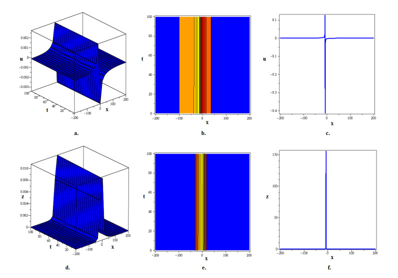
I investigated soliton phenomena in a prominent nonlinear fractional partial differential equation (FPDE) namely the conformable coupled Drinfeld-Sokolov-Wilson system (CCDSWS) using a novel variant of the novel extended direct algebraic method (EDAM), namely $ r $+mEDAM. The conformable fractional derivatives are used to generalize the model due to the memory and hereditary features that are inherent in the fractional dynamics. The model was initially transformed into a more manageable system of integer-order nonlinear ordinary differential equations (NODEs) through the implementation of complex transformation. The obtained system of NODEs is further transformed into a system of algebraic equations, which yields, by solving new plethora of soliton solutions for CCDSWS in the form of generalized trigonometrical, exponential hyperbolical, and rational functions. Moreover, we employed 2D, 3D, and contour graphics to show the behavior of acquired solitons, making it abundantly evident that the obtained solitons take the shape of kink, anti-kink, bright, dark, bright-dark, and bell-shaped kink solitons within the framework of CCDSWS. The results confirmed the efficiency of the presented approach in finding solitonic solutions, which in its turn expands knowledge of nonlinear FPDEs. The aimed to theoretical and application perspectives in fractional solitons applicable in areas such fluid mechanics, plasma physic, optical communications, etc.

| [1] | T. Roubíček, Nonlinear partial differential equations with applications, Birkhäuser Basel, Vol. 153, 2013. https://doi.org/10.1007/978-3-0348-0513-1 |
| [2] | L. Debnath, Nonlinear partial differential equations for scientists and engineers, 2 Eds., Birkhäuser Boston, 2005. https://doi.org/10.1007/b138648 |
| [3] | D. Cioranescu, J. L. Lions, Nonlinear partial differential equations and their applications, College de France Seminar Volume XIV, 1 Ed., Elsevier, 2002. |
| [4] | W. F. Ames, Nonlinear partial differential equations in engineering, Vol. 18, Academic press, 1965. |
| [5] | J. L. Kazdan, Applications of partial differential equations to problems in geometry, Graduate Texts in Mathematics, 1983. |
| [6] |
A. P. Bassom, P. A. Clarkson, A. C. Hicks, On the application of solutions of the fourth Painlevé equation to various physically motivated nonlinear partial differential equations, Adv. Differ. Equ., 1 (1996), 175–198. https://doi.org/10.57262/ade/1366896236 doi: 10.57262/ade/1366896236

|
| [7] |
H. Khan, R. Shah, J. F. Gómez-Aguilar, D. Baleanu, P. Kumam, Travelling waves solution for fractional-order biological population model, Math. Model. Nat. Phenom., 16 (2021), 32. https://doi.org/10.1051/mmnp/2021016 doi: 10.1051/mmnp/2021016
|
| [8] | B. Barnes, E. Osei-Frimpong, F. O. Boateng, J. Ackora-Prah, A two-dimensional chebyshev wavelet method for solving partial differential equations, J. Math. Theory Model., 6 (2016), 124–138. |
| [9] | M. Khalid, M. Sultana, F. Zaidi, U. Arshad, An Elzaki transform decomposition algorithm applied to a class of non-linear differential equations, J. Nat. Sci. Res., 5 (2015), 48–56. |
| [10] |
M. Kumar, Umesh, Recent development of Adomian decomposition method for ordinary and partial differential equations, Int. J. Appl. Comput. Math., 8 (2022), 81. https://doi.org/10.1007/s40819-022-01285-6 doi: 10.1007/s40819-022-01285-6
|
| [11] | H. Gündoǧdu, Ö. F. Gözükızıl, Solving nonlinear partial differential equations by using Adomian decomposition method, modified decomposition method and Laplace decomposition method, MANAS J. Eng., 5 (2017), 1–13. |
| [12] |
S. Momani, Z. Odibat, Homotopy perturbation method for nonlinear partial differential equations of fractional order, Phys. Lett. A, 365 (2007), 345–350. https://doi.org/10.1016/j.physleta.2007.01.046 doi: 10.1016/j.physleta.2007.01.046
|
| [13] |
H. Khan, S. Barak, P. Kumam, M. Ariff, Analytical solutions of fractional Klein-Gordon and gas dynamics equations, via the $(G'/G)$-expansion method, Symmetry, 11 (2019), 566. https://doi.org/10.3390/sym11040566 doi: 10.3390/sym11040566
|
| [14] |
R. Shah, H. Khan, P. Kumam, M. Arif, D. Baleanu, Natural transform decomposition method for solving fractional-order partial differential equations with proportional delay, Mathematics, 7 (2019), 532. https://doi.org/10.3390/math7060532 doi: 10.3390/math7060532
|
| [15] |
R. Ali, E. Tag-eldin, A comparative analysis of generalized and extended $(\frac {G'}{G})$-expansion methods for travelling wave solutions of fractional Maccari's system with complex structure, Alex. Eng. J., 79 (2023), 508–530. https://doi.org/10.1016/j.aej.2023.08.007 doi: 10.1016/j.aej.2023.08.007
|
| [16] |
M. Kamrujjaman, A. Ahmed, J. Alam, Travelling waves: interplay of low to high Reynolds number and tan-cot function method to solve Burger's equations, J. Appl. Math. Phys., 7 (2019), 861–873. https://doi.org/10.4236/jamp.2019.74058 doi: 10.4236/jamp.2019.74058
|
| [17] |
M. Cinar, A. Secer, M. Ozisik, M. Bayram, Derivation of optical solitons of dimensionless Fokas-Lenells equation with perturbation term using Sardar sub-equation method, Opt. Quant. Electron., 54 (2022), 402. https://doi.org/10.1007/s11082-022-03819-0 doi: 10.1007/s11082-022-03819-0
|
| [18] | M. S. Islam, K. Khan, M. A. Akbar, The generalized Kudrysov method to solve some coupled nonlinear evolution equations, Asian J. Math. Comput. Res., 3 (2015), 104–121. |
| [19] |
A. Bekir, E. Aksoy, A. C. Cevikel, Exact solutions of nonlinear time fractional partial differential equations by sub-equation method, Math. Methods Appl. Sci., 38 (2015), 2779–2784. https://doi.org/10.1002/mma.3260 doi: 10.1002/mma.3260
|
| [20] |
S. Bibi, S. T. Mohyud-Din, U. Khan, N. Ahmed, Khater method for nonlinear Sharma Tasso-Olever (STO) equation of fractional order, Results Phys., 7 (2017), 4440–4450. https://doi.org/10.1016/j.rinp.2017.11.008 doi: 10.1016/j.rinp.2017.11.008
|
| [21] |
M. Dehghan, J. Manafian Heris, A. Saadatmandi, Application of the exp-function method for solving a partial differential equation arising in biology and population genetics, Int. J. Numer. Methods Heat Fluid Flow, 21 (2011), 736–753. https://doi.org/10.1108/09615531111148482 doi: 10.1108/09615531111148482
|
| [22] |
S. Noor, A. S. Alshehry, A. Khan, I. Khan, Analysis of soliton phenomena in $(2+ 1)$-dimensional Nizhnik-Novikov-Veselov model via a modified analytical technique, AIMS Math., 8 (2023), 28120–28142. https://doi.org/10.3934/math.20231439 doi: 10.3934/math.20231439
|
| [23] |
H. Yasmin, N. H. Aljahdaly, A. M. Saeed, R. Shah, Investigating symmetric soliton solutions for the fractional coupled Konno-Onno system using improved versions of a novel analytical technique, Mathematics, 11 (2023), 2686. https://doi.org/10.3390/math11122686 doi: 10.3390/math11122686
|
| [24] |
R. Ali, M. M. Alam, S. Barak, Exploring chaotic behavior of optical solitons in complex structured conformable perturbed Radhakrishnan-Kundu-Lakshmanan model, Phys. Scr., 99 (2024), 095209. https://doi.org/10.1088/1402-4896/ad67b1 doi: 10.1088/1402-4896/ad67b1
|
| [25] |
M. Iqbal, W. A. Faridi, R. Ali, A. R. Seadawy, A. A. Rajhi, A. E. Anqi, et al., Dynamical study of optical soliton structure to the nonlinear Landau-Ginzburg-Higgs equation through computational simulation, Opt. Quant. Electron., 56 (2024), 1192. https://doi.org/10.1007/s11082-024-06401-y doi: 10.1007/s11082-024-06401-y
|
| [26] |
R. Ali, Z. Zhang, H. Ahmad, M. M. Alam, The analytical study of soliton dynamics in fractional coupled Higgs system using the generalized Khater method, Opt. Quant. Electron., 56 (2024), 1067. https://doi.org/10.1007/s11082-024-06924-4 doi: 10.1007/s11082-024-06924-4
|
| [27] |
S. Noor, A. S. Alshehry, H. M. Dutt, R. Nazir, A. Khan, R. Shah, Investigating the dynamics of time-fractional Drinfeld-Sokolov-Wilson system through analytical solutions, Symmetry, 15 (2023), 703. https://doi.org/10.3390/sym15030703 doi: 10.3390/sym15030703
|
| [28] |
X. Z. Zhang, M. I. Asjad, W. A. Faridi, A. Jhangeer, M. İnç, The comparative report on dynamical analysis about fractional nonlinear Drinfeld-Sokolov-Wilson systemm, Fractals, 30 (2022), 2240138. https://doi.org/10.1142/S0218348X22401387 doi: 10.1142/S0218348X22401387
|
| [29] |
V. G. Drinfel'd, V. V. Sokolov, Lie algebras and equations of Korteweg-de Vries type, J. Math. Sci., 30 (1985), 1975–2036. https://doi.org/10.1007/BF02105860 doi: 10.1007/BF02105860
|
| [30] |
G. Wilson, The affine Lie algebra ${C^{(1)}}_2$ and an equation of Hirota and Satsuma, Phys. Lett. A, 89 (1982), 332–334. https://doi.org/10.1016/0375-9601(82)90186-4 doi: 10.1016/0375-9601(82)90186-4
|
| [31] |
R. Arora, A. Kumar, Solution of the coupled Drinfeld's-Sokolov-Wilson (DSW) system by homotopy analysis method, Adv. Sci. Eng. Med., 5 (2013), 1105–1111. https://doi.org/10.1166/asem.2013.1399 doi: 10.1166/asem.2013.1399
|
| [32] |
M. Usman, A. Hussain, F. D. Zaman, S. M. Eldin, Symmetry analysis and exact Jacobi elliptic solutions for the nonlinear couple Drinfeld Sokolov Wilson dynamical system arising in shallow water wavess, Results Phys., 51 (2023), 106613. https://doi.org/10.1016/j.rinp.2023.106613 doi: 10.1016/j.rinp.2023.106613
|
| [33] |
J. Singh, D. Kumar, D. Baleanu, S. Rathore, An efficient numerical algorithm for the fractional Drinfeld-Sokolov-Wilson equation, Appl. Math. Comput., 335 (2018), 12–24. https://doi.org/10.1016/j.amc.2018.04.025 doi: 10.1016/j.amc.2018.04.025
|
| [34] |
V. E. Tarasov, On chain rule for fractional derivatives, Commun. Nonlinear Sci. Numer. Simul., 30 (2016), 1–4. https://doi.org/10.1016/j.cnsns.2015.06.007 doi: 10.1016/j.cnsns.2015.06.007
|
| [35] |
J. H. He, S. K. Elagan, Z. B. Li, Geometrical explanation of the fractional complex transform and derivative chain rule for fractional calculus, Phys. Lett. A, 376 (2012), 257–259. https://doi.org/10.1016/j.physleta.2011.11.030 doi: 10.1016/j.physleta.2011.11.030
|
| [36] | M. Z. Sarıkaya, H. Budak, H. Usta, On generalized the conformable fractional calculus, TWMS J. Appl. Eng. Math., 9 (2019), 792–799. |


Figures(5)

Naher Mohammed A. Alsafri. Solitonic behaviors in the coupled Drinfeld-Sokolov-Wilson system with fractional dynamics[J]. AIMS Mathematics, 2025, 10(3): 4747-4774. doi: 10.3934/math.2025218


 DownLoad: