Exponential stability of ARZ traffic flow model based on $ 2\times 2 $ variable-coefficient hyperbolic system

Yiyan Wang; Dongxia Zhao; Caifen Sun; Yaping Guo; Yiyan Wang; Dongxia Zhao; Caifen Sun; Yaping Guo

doi:10.3934/math.2025026

AIMS Mathematics

2025, Volume 10, Issue 1: 584-597. doi: 10.3934/math.2025026

Previous Article Next Article

Research article

Exponential stability of ARZ traffic flow model based on $ 2\times 2 $ variable-coefficient hyperbolic system

1.
School of Mathematics, North University of China, Taiyuan 030051, China
2.
School of Mathematical Sciences, Shanxi University, Taiyuan 030006, China

Received: 26 November 2024 Revised: 23 December 2024 Accepted: 27 December 2024 Published: 10 January 2025
MSC : 34H05, 35L60, 93D15

This paper studies the exponential stability of the Aw-Rascle-Zhang (ARZ) traffic flow model. Given that the steady state may be non-uniform, we obtain a $ 2\times2 $ hyperbolic system with variable coefficients. Then, by combining ramp metering and variable speed limit control, we deduce a kind of proportional boundary feedback controller. The well-posedness of the closed-loop system is proved by using the theory of semigroups of operators. Moreover, a novel Lyapunov function, whose weighted function is constructed by the solution of a first-order ordinary differential equation, can be used for the stability analysis. The analysis gives a sufficient stability condition for the feedback parameters, which is easy to verify. Finally, the effectiveness of boundary control and the feasibility of the feedback parameters are obtained by numerical simulation.
- boundary feedback control,
- exponential stability,
- Lyapunov function,
- traffic flow model,
- variable-coefficient hyperbolic system
Citation: Yiyan Wang, Dongxia Zhao, Caifen Sun, Yaping Guo. Exponential stability of ARZ traffic flow model based on $ 2\times 2 $ variable-coefficient hyperbolic system[J]. AIMS Mathematics, 2025, 10(1): 584-597. doi: 10.3934/math.2025026

Related Papers:

Abstract

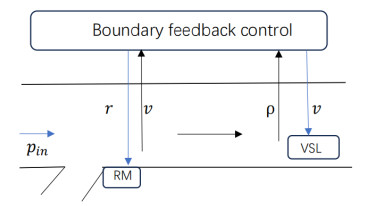
This paper studies the exponential stability of the Aw-Rascle-Zhang (ARZ) traffic flow model. Given that the steady state may be non-uniform, we obtain a $ 2\times2 $ hyperbolic system with variable coefficients. Then, by combining ramp metering and variable speed limit control, we deduce a kind of proportional boundary feedback controller. The well-posedness of the closed-loop system is proved by using the theory of semigroups of operators. Moreover, a novel Lyapunov function, whose weighted function is constructed by the solution of a first-order ordinary differential equation, can be used for the stability analysis. The analysis gives a sufficient stability condition for the feedback parameters, which is easy to verify. Finally, the effectiveness of boundary control and the feasibility of the feedback parameters are obtained by numerical simulation.

References

[1]	A. Aw, M. Rascle, Resurrection of "second order" models of traffic flow, SIAM J. Appl. Math., 60 (2000), 916–938. https://doi.org/10.1137/S0036139997332099 doi: 10.1137/S0036139997332099
[2]	H. M. Zhang, A non–equilibrium traffic model devoid of gas-like behavior, Transport. Res. B-Meth., 36 (2002), 275–290. https://doi.org/10.1016/S0191-2615(00)00050-3 doi: 10.1016/S0191-2615(00)00050-3
[3]	J. M. Greenberg, L. T. Tsien, The effect of boundary damping for the quasilinear wave equation, J. Differ. Equ., 52 (1984), 66–75. https://doi.org/10.1016/0022-0396(84)90135-9 doi: 10.1016/0022-0396(84)90135-9
[4]	J. M. Coron, B. d'Andréa-Novel, G. Bastia, A Lyapunov approach to control irrigation canals modeled by Saint-Venant equations, In: 1999 European Control Conference, 1999, 3178–3183. https://doi.org/10.23919/ECC.1999.7099816
[5]	H. Zhao, J. Zhan, L. Zhang, Saturated boundary feedback stabilization for LWR traffic flow model, Syst. Control Lett., 173 (2023), 105465. https://doi.org/10.1016/j.sysconle.2023.105465 doi: 10.1016/j.sysconle.2023.105465
[6]	C. Prieur, J. J. Winkin, Boundary feedback control of linear hyperbolic systems: Application to the Saint-Venant-Exner equations, Automatica, 89 (2018), 44–51. https://doi.org/10.1016/j.automatica.2017.11.028 doi: 10.1016/j.automatica.2017.11.028
[7]	K. Wang, Z. Wang, W. Yao, Boundary feedback stabilization of quasilinear hyperbolic systems with partially dissipative structure, Syst. Control Lett., 146 (2020), 104815. https://doi.org/10.1016/j.sysconle.2020.104815 doi: 10.1016/j.sysconle.2020.104815
[8]	L. Zhang, C. Prieur, J. Qiao, Local proportional-integral boundary feedback stabilization for quasilinear hyperbolic systems of balance laws, SIAM J. Control Optim., 58 (2020), 2143–2170. https://doi.org/10.1137/18M1214883 doi: 10.1137/18M1214883
[9]	D. Zhao, D. Fan, Y. Guo, The spectral analysis and exponential stability of a 1-d $2\times 2$ Hyperbolic system with proportional feedback control, Int. J. Control, Autom. Syst., 20 (2022), 2633–2640. http://dx.doi.org/10.1007/s12555-021-0507-0 doi: 10.1007/s12555-021-0507-0
[10]	A. Hayat, P. Shang, A quadratic Lyapunov function for Saint-Venant equations with arbitrary friction and space varying slope, Automatica, 100 (2019), 52–60. https://doi.org/10.1016/j.automatica.2018.10.035 doi: 10.1016/j.automatica.2018.10.035
[11]	A. Hayat, Y. Hu, P. Shang, PI control for the cascade channels modeled by general Saint-Venant equations, IEEE Trans. Automat. Control, 69 (2024), 4974–4987. https://doi.org/10.1109/TAC.2023.3341767 doi: 10.1109/TAC.2023.3341767
[12]	J. Qi, S. Mo, M. Krstic, Delay-compensated distributed PDE control of traffic with connected/automated vehicles, IEEE Trans. Automat. Control, 68 (2023), 2229–2244. https://doi.org/10.1109/TAC.2022.3174032 doi: 10.1109/TAC.2022.3174032
[13]	J. Zeng, Y. Qian, F. Yin, L. Zhu, D. Xu, A multi-value cellular automata model for multi-lane traffic flow under lagrange coordinate, Comput. Math. Organ. Theory, 28 (2022), 178–192. https://doi.org/10.1007/s10588-021-09345-w doi: 10.1007/s10588-021-09345-w
[14]	Z. Li, C. Xu, D. Li, W. Wang, Comparing the effects of ramp metering and variable speed limit on reducing travel time and crash risk at bottlenecks, IET Intell. Transp. Syst., 12 (2018), 120–126. https://doi.org/10.1049/iet-its.2017.0064 doi: 10.1049/iet-its.2017.0064
[15]	J. R. D. Frejo, B. De Schutter, Logic-based traffic flow control for ramp metering and variable speed limits-Part 1: Controller, IEEE Trans. Intell. Transp. Syst., 22 (2021), 2647–2657. https://doi.org/10.1109/TITS.2020.2973717 doi: 10.1109/TITS.2020.2973717
[16]	Z. He, L. Wang, Z. Su, W. Ma, Integrating variable speed limit and ramp metering to enhance vehicle group safety and efficiency in a mixed traffic environment, Phys. A, 641 (2024), 129754. https://doi.org/10.1016/j.physa.2024.129754 doi: 10.1016/j.physa.2024.129754
[17]	H. Yu, M. Krstic, Traffic congestion control for Aw-Rascle-Zhang model, Automatica, 100 (2019), 38–51. https://doi.org/10.1016/j.automatica.2018.10.040 doi: 10.1016/j.automatica.2018.10.040
[18]	H. Yu, J. Auriol, M. Krstic, Simultaneous downstream and upstream output-feedback stabilization of cascaded freeway traffic, Automatica, 136 (2022), 110044. https://doi.org/10.1016/j.automatica.2021.110044 doi: 10.1016/j.automatica.2021.110044
[19]	N. Espitia, J. Auriol, H. Yu, M. Krstic, Traffic flow control on cascaded roads by event‐triggered output feedback, Int. J. Robust Nonlin., 32 (2022), 5919–5949. https://doi.org/10.1002/rnc.6122 doi: 10.1002/rnc.6122
[20]	N. Espitia, H. Yu, M. Krstic, Event-triggered varying speed limit control of stop-and-go traffic, IFAC-PapersOnLine, 53 (2020), 7509–7514. https://doi.org/10.1016/j.ifacol.2020.12.1343 doi: 10.1016/j.ifacol.2020.12.1343
[21]	H. Yu, M. Krstic, Output feedback control of two-lane traffic congestion, Automatica, 125 (2021), 109379. https://doi.org/10.1016/j.automatica.2020.109379 doi: 10.1016/j.automatica.2020.109379
[22]	S. C. Vishnoi, S. A. Nugroho, A. F. Taha, C. G. Claudel, Traffic state estimation for connected vehicles using the second-order aw-rascle-zhang traffic model, IEEE T. Intell. Transp., 25 (2024), 16719–16733. https://doi.org/10.1109/TITS.2024.3420438 doi: 10.1109/TITS.2024.3420438
[23]	P. Zhang, B. Rathnayake, M. Diagne, M. Krstic, Performance-barrier-based event-triggered boundary control of congested ARZ traffic PDEs, IFAC-PapersOnLine, 58 (2024), 182–187. https://doi.org/10.1016/j.ifacol.2024.07.337 doi: 10.1016/j.ifacol.2024.07.337
[24]	L. Zhang, H. Luan, Y. Lu, C. Prieur, Boundary feedback stabilization of freeway traffic networks: ISS control and experiments, IEEE Trans. Control Syst. Technol., 30 (2022), 997–1008. https://doi.org/10.1109/TCST.2021.3088093 doi: 10.1109/TCST.2021.3088093
[25]	L. Zhang, C. Prieur, J. Qiao, PI boundary control of linear hyperbolic balance laws with stabilization of ARZ traffic flow models, Syst. Control Lett., 123 (2019), 85–91. https://doi.org/10.1016/j.sysconle.2018.11.005 doi: 10.1016/j.sysconle.2018.11.005

Reader Comments

Your name:*

Email:*
© 2025 the Author(s), licensee AIMS Press. This is an open access article distributed under the terms of the Creative Commons Attribution License (http://creativecommons.org/licenses/by/4.0)