Agricultural decision-making involves a complex process of choosing strategies and options to enhance resource utilization, overall productivity, and farming practices. Agricultural stakeholders and farmers regularly make decisions at various levels of the farm cycle, ranging from crop selection and planting to harvesting and marketing. In agriculture, where crop health has played a central role in economic and yield outcomes, incorporating deep learning (DL) techniques has developed as a transformative force for the decision-making process. DL techniques, with their capability to discern subtle variations and complex patterns in plant health, empower agricultural experts and farmers to make informed decisions based on data-driven, real-time insights. Thus, we presented a Bayesian optimizer with deep learning based pepper leaf disease detection for decision making (BODL-PLDDM) approach in the agricultural sector. The BODL-PLDDM technique aimed to identify the healthy and bacterial spot pepper leaf disease. Primarily, the BODL-PLDDM technique involved a Wiener filtering (WF) approach for pre-processing. Besides, the complex and intrinsic feature patterns could be extracted using the Inception v3 model. Also, the Bayesian optimization (BO) algorithm was used for the optimal hyperparameter selection process. For disease detection, a crayfish optimization algorithm (COA) with a long short-term memory (LSTM) method was employed to identify the precise presence of pepper leaf diseases. The experimentation validation of the BODL-PLDDM system was verified using the Plant Village dataset. The obtained outcomes underlined the promising detection results of the BODL-PLDDM technique over other existing methods.
Citation: Asma A Alhashmi, Manal Abdullah Alohali, Nazir Ahmad Ijaz, Alaa O. Khadidos, Omar Alghushairy, Ahmed Sayed. Bayesian optimization with deep learning based pepper leaf disease detection for decision-making in the agricultural sector[J]. AIMS Mathematics, 2024, 9(7): 16826-16847. doi: 10.3934/math.2024816
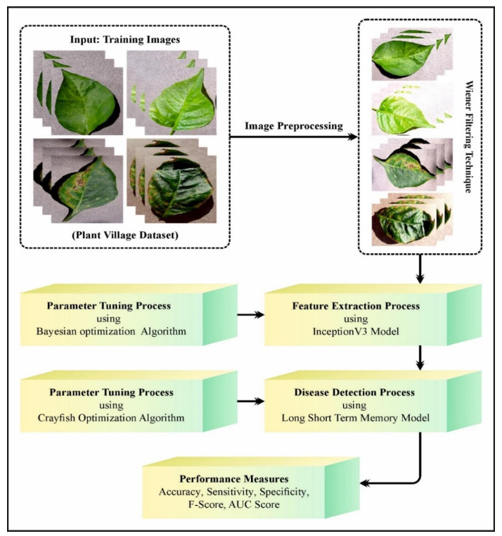
Agricultural decision-making involves a complex process of choosing strategies and options to enhance resource utilization, overall productivity, and farming practices. Agricultural stakeholders and farmers regularly make decisions at various levels of the farm cycle, ranging from crop selection and planting to harvesting and marketing. In agriculture, where crop health has played a central role in economic and yield outcomes, incorporating deep learning (DL) techniques has developed as a transformative force for the decision-making process. DL techniques, with their capability to discern subtle variations and complex patterns in plant health, empower agricultural experts and farmers to make informed decisions based on data-driven, real-time insights. Thus, we presented a Bayesian optimizer with deep learning based pepper leaf disease detection for decision making (BODL-PLDDM) approach in the agricultural sector. The BODL-PLDDM technique aimed to identify the healthy and bacterial spot pepper leaf disease. Primarily, the BODL-PLDDM technique involved a Wiener filtering (WF) approach for pre-processing. Besides, the complex and intrinsic feature patterns could be extracted using the Inception v3 model. Also, the Bayesian optimization (BO) algorithm was used for the optimal hyperparameter selection process. For disease detection, a crayfish optimization algorithm (COA) with a long short-term memory (LSTM) method was employed to identify the precise presence of pepper leaf diseases. The experimentation validation of the BODL-PLDDM system was verified using the Plant Village dataset. The obtained outcomes underlined the promising detection results of the BODL-PLDDM technique over other existing methods.

| [1] | R. Sharma, K. Vinay, D. Bordoloi, Deep learning meets agriculture: A faster RCNN based approach to pepper leaf blight disease detection and multi-classification, In: 2023 4th International Conference for Emerging Technology (INCET), 2023. |
| [2] | M. B. Devi, K. Amarendra, Machine learning-based application to detect pepper leaf diseases using histgradientboosting classifier with fused HOG and LBP features, In: Smart Technologies in Data Science and Communication: Proceedings of SMART-DSC, Singapore: Springer, 2021. |
| [3] | T. H. H. Aldhyani, A. Hasan, R. J. Eunice, D. J. Hemanth, Leaf pathology detection in potato and pepper bell plant using convolutional neural networks, In: 2022 7th International Conference on Communication and Electronics Systems (ICCES), 2022. |
| [4] | C. H. Kim, M. N. R. Samsuzzaman, K. Y. Lee, M. R. Ali, Deep learning-based identification of Pepper (Capsicum annuum L.) diseases: A review, Precis. Agric., 5 (2023), 68. |
| [5] | A. S. Kini, K. V. Prema, S. N. Pai, State of the art deep learning implementation for multiclass classification of black pepper leaf diseases, 2023. https://doi.org/10.21203/rs.3.rs-3272019/v1 |
| [6] | I. Haque, M. A. Islam, K. Roy, M. M. Rahaman, A. A. Shohan, I. Md Saiful, Classifying pepper disease based on transfer learning: A deep learning approach, In: 2022 International Conference on Applied Artificial Intelligence and Computing (ICAAIC), 2022. http://doi.org/10.1109/ICAAIC53929.2022.9793178 |
| [7] | K. Andersson, M. S. Hoassain, Bell pepper leaf disease classification using convolutional neural network, In: Intelligent Computing & Optimization: Proceedings of the 5th International Conference on Intelligent Computing and Optimization 2022 (ICO2022), Springer Nature, 569 (2022). |
| [8] | Y. Akhalifi, A. Subekti, Bell pepper leaf disease classification using fine-tuned transfer learning, J. Elektronikadan Telekomunikasi, 23 (2023), 55–61. |
| [9] | P. Thakur, C. Anuradha, A. P. Singh, Plant disease detection of bell pepper plant using transfer learning over different models, In: 2021 8th International Conference on Signal Processing and Integrated Networks (SPIN), 2021,384–389. |
| [10] | C. Y. Khew, Y. Q. Teow, E. T. Lau, S. S. Hwang, C. H. Bong, N. K. Lee, Evaluation of deep learning for image-based black pepper disease and nutrient deficiency classification, In: 2021 2nd International Conference on Artificial Intelligence and Data Sciences (AiDAS), 2021, 1–6. http://doi.org/10.1109/AiDAS53897.2021.9574346 |
| [11] | I. Bouacida, B. Farou, L. Djakhdjakha, H. Seridi, M. Kurulay, Innovative deep learning approach for cross-crop plant disease detection: A generalized method for identifying unhealthy leaves, Inform. Process. Agricul., 2024. |
| [12] | M. Shoaib, T. Hussain, B. Shah, I. Ullah, S. M. Shah, F. Ali, et al., Deep learning-based segmentation and classification of leaf images for detection of tomato plant disease, Front. Plant Sci., 13 (2022), 1031748. |
| [13] | Y. A. Bezabih, A. O. Salau, B. M. Abuhayi, A. A. Mussa, A. M. Ayalew, CPD-CCNN: Classification of pepper disease using a concatenation of convolutional neural network models, Sci. Rep., 13 (2023), 15581. |
| [14] | S. S. A. Begum, H. Syed, GSAtt-CMNetV3: Pepper leaf disease classification using osprey optimization, IEEE Access, 2024. |
| [15] | D. I. Lee, J. H. Lee, S. H. Jang, S. J. Oh, I. C. Doo, Crop disease diagnosis with deep learning-based image captioning and object detection, Appl. Sci., 13 (2023), 3148. |
| [16] | V. Gautam, R. K. Ranjan, P. Dahiya, A. Kumar, ESDNN: A novel ensembled stack deep neural network for mango leaf disease classification and detection, Multimed. Tools Appl., 83 (2024), 10989–11015. |
| [17] | S. Ashwinkumar, S. Rajagopal, V. Manimaran, B. Jegajothi, Automated plant leaf disease detection and classification using optimal MobileNet based convolutional neural networks, Mater. Today Proceed., 51 (2022), 480–487. |
| [18] | A. Kumar, V. K. Patel, Classification and identification of disease in potato leaf using hierarchical based deep learning convolutional neural network, Multimed. Tools Appl., 2023, 1–27. |
| [19] | N. Krishnamoorthy, L. N. Prasad, C. P. Kumar, B. Subedi, H. B. Abraha, V. E. Sathishkumar, Rice leaf diseases prediction using deep neural networks with transfer learning, Environ. Res., 198 (2021), 111275. |
| [20] |
M. Subramanian, N. P. Lv, S. VE, Hyperparameter optimization for transfer learning of VGG16 for disease identification in corn leaves using Bayesian optimization, Big Data, 10 (2022), 215–229. https://doi.org/10.1089/big.2021.021 doi: 10.1089/big.2021.021

|
| [21] |
J. V. Valls, D. Vivet, E. Chaumette, F. Vincent, P. Closas, Recursive linearly constrained Wiener filter for robust multi-channel signal processing, Signal Process., 167 (2020), 107291. https://doi.org/10.1016/j.sigpro.2019.107291 doi: 10.1016/j.sigpro.2019.107291
|
| [22] |
K. S. Rao, P. V. Terlapu, D. Jayaram, K. K. Raju, G. K. Kumar, R. Pemula, et al., Intelligent ultrasound imaging for enhanced breast cancer diagnosis: Ensemble transfer learning strategies, IEEE Access, 2024. http://doi.org/10.1109/ACCESS.2024.3358448 doi: 10.1109/ACCESS.2024.3358448
|
| [23] |
A. Riboni, N. Ghioldi, A. Candelieri, M. Borrotti, Bayesian optimization and deep learning for steering wheel angle prediction, Sci. Rep., 12 (2022), 8739. https://doi.org/10.1038/s41598-022-12509-6 doi: 10.1038/s41598-022-12509-6
|
| [24] |
A. Cuk, T. Bezdan, L. Jovanovic, M. Antonijevic, M. Stankovic, V. Simic, et al., Tuning attention based long-short term memory neural networks for Parkinson's disease detection using modified metaheuristics, Sci. Rep., 14 (2024), 4309. https://doi.org/10.1038/s41598-024-54680-y doi: 10.1038/s41598-024-54680-y
|
| [25] |
A. Sagheer, M. Kotb, Unsupervised pre-training of a deep LSTM-based stacked autoencoder for multivariate time series forecasting problems, Sci. Rep., 9 (2019), 19038. https://doi.org/10.1038/s41598-019-55320-6 doi: 10.1038/s41598-019-55320-6
|
| [26] | Plant Village dataset. Available from: https://www.kaggle.com/datasets/adilmubashirchaudhry/plant-village-dataset. |


Figures(16) / Tables(4)

Asma A Alhashmi, Manal Abdullah Alohali, Nazir Ahmad Ijaz, Alaa O. Khadidos, Omar Alghushairy, Ahmed Sayed. Bayesian optimization with deep learning based pepper leaf disease detection for decision-making in the agricultural sector[J]. AIMS Mathematics, 2024, 9(7): 16826-16847. doi: 10.3934/math.2024816


 DownLoad: