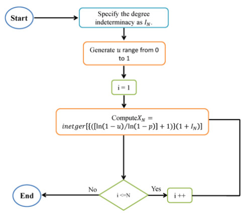
This paper introduces the geometric distribution in the context of neutrosophic statistics. The research outlines the essential properties of this new distribution and introduces novel algorithms for generating imprecise geometric data. The study explores the practical applications of this distribution in the industry, highlighting differences in data generated under deterministic and indeterminate conditions using detailed tables, simulation studies, and real-world applications. The results indicate that the level of uncertainty has a substantial impact on data generation from the geometric distribution. These findings suggest updating classical statistical algorithms to better handle the generation of imprecise data. Therefore, decision-makers should exercise caution when using data from the geometric distribution in uncertain environments.
Citation: Muhammad Aslam, Mohammed Albassam. Neutrosophic geometric distribution: Data generation under uncertainty and practical applications[J]. AIMS Mathematics, 2024, 9(6): 16436-16452. doi: 10.3934/math.2024796
This paper introduces the geometric distribution in the context of neutrosophic statistics. The research outlines the essential properties of this new distribution and introduces novel algorithms for generating imprecise geometric data. The study explores the practical applications of this distribution in the industry, highlighting differences in data generated under deterministic and indeterminate conditions using detailed tables, simulation studies, and real-world applications. The results indicate that the level of uncertainty has a substantial impact on data generation from the geometric distribution. These findings suggest updating classical statistical algorithms to better handle the generation of imprecise data. Therefore, decision-makers should exercise caution when using data from the geometric distribution in uncertain environments.

| [1] | M. Beria, Confidence interval estimation for a geometric distribution, UNLV Retrospective Theses & Dissertations, 2015 (2005), 1924. http://doi.org/10.25669/too9-2lgp |
| [2] | F. Y. Chen, The goodness-of-fit tests for geometric models, Dissertations, 2013 (2013), 350. https://digitalcommons.njit.edu/dissertations/350 |
| [3] | L. Bertoli-Barsotti, T. Lando, A geometric model for the analysis of citation distributions, International Journal of Mathematical Models and Methods in Applied Sciences, 9 (2015), 315–319. |
| [4] | A. Slim, G. L. Heileman, M. Hickman and C. T. Abdallah, A geometric distributed probabilistic model to predict graduation rates, 2017 IEEE SmartWorld, Ubiquitous Intelligence & Computing, Advanced & Trusted Computed, Scalable Computing & Communications, Cloud & Big Data Computing, Internet of People and Smart City Innovation (SmartWorld/SCALCOM/UIC/ATC/CBDCom/IOP/SCI), San Francisco, CA, USA, 2017, 1–8. http://doi.org10.1109/UIC-ATC.2017.8397646 |
| [5] | W. K. Gao, An extended geometric process and its application in replacement policy, P. I. Mech. Eng. O-J. Ris., 234 (2020), 88–103. http://doi.org10.1177/1748006X19868891 |
| [6] | E. Altun, A new generalization of geometric distribution with properties and applications, Commun. Stat.-Simul. C., 49 (2020), 793–807. https://doi.org/10.1080/03610918.2019.1639739 |
| [7] | M. M. A. Almazah, T. Erbayram, Y. Akdoğan, M. M. A. Sobhi, A. Z. Afify, A new extended geometric distribution: properties, regression model, and actuarial applications, Mathematics, 9 (2021), 1336. http://doi.org10.3390/math9121336 |
| [8] | Z. Y. Zhang, X. T. Tang, Q. Huang, W. J. Lee, Preemptive medium-low voltage arc flash detection with geometric distribution analysis on magnetic field, IEEE T. Ind. Appl., 57 (2021), 2129–2137. http://doi.org10.1109/TIA.2021.3057314 |
| [9] | I. Ghosh, F. Marques, S. Chakraborty, A bivariate geometric distribution via conditional specification: properties and applications, Commun. Stat.-Simul. C., 52 (2023), 5925–5945. http://doi.org10.1080/03610918.2021.2004419 |
| [10] | N. Abbas, On classical and Bayesian reliability of systems using bivariate generalized geometric distribution, J. Stat. Theory Appl., 22 (2023), 151–169. https://doi.org/10.1007/s44199-023-00058-4 |
| [11] | Y. Akdoğan, C. Kuş, A. Asgharzadeh, İ. Kınacı, F. Sharafi, Uniform-geometric distribution, J. Stat. Comput. Sim., 86 (2016), 1754–1770. http://doi.org10.1080/00949655.2015.1081907 |
| [12] | S. Nadarajah, S. A. A. Bakar, An exponentiated geometric distribution, Appl. Math. Model., 40 (2016), 6775–6784. https://doi.org/10.1016/j.apm.2015.11.010 |
| [13] | A. S. Hassan, M. A. Abdelghafar, Exponentiated Lomax geometric distribution: properties and applications, Pak. J. Stat. Oper. Res., 13 (2017), 545–566. https://doi.org/10.18187/pjsor.v13i3.1437 |
| [14] | A. T. Ramadan, A. H. Tolba, B. S. El-Desouky, A unit half-logistic geometric distribution and its application in insurance, Axioms, 11 (2022), 676. https://doi.org/10.3390/axioms11120676 |
| [15] | F. Smarandache, Introduction to neutrosophic statistics: infinite study, Columbus: Romania-Educational Publisher, 2014. http://doi.org10.13140/2.1.2780.1289 |
| [16] | F. Smarandache, Neutrosophic statistics is an extension of interval statistics, while Plithogenic statistics is the most general form of statistics (second version), International Journal of Neutrosophic Science, 19 (2022), 148–165. http://doi.org10.54216/IJNS.190111 |
| [17] | J. Q. Chen, J. Ye, S. G. Du, Scale effect and anisotropy analyzed for neutrosophic numbers of rock joint roughness coefficient based on neutrosophic statistics, Symmetry, 9 (2017), 208. https://doi.org/10.3390/sym9100208 |
| [18] | J. Q. Chen, J. Ye, S. G. Du, R. Yong, Expressions of rock joint roughness coefficient using neutrosophic interval statistical numbers, Symmetry, 9 (2017), 123. https://doi.org/10.3390/sym9070123 |
| [19] | W. Q. Duan, Z. Khan, M. Gulistan, A. Khurshid, Neutrosophic exponential distribution: modeling and applications for complex data analysis, Complexity, 2021 (2021), 5970613. https://doi.org/10.1155/2021/5970613 |
| [20] | C. Granados, Some discrete neutrosophic distributions with neutrosophic parameters based on neutrosophic random variables, Hacet. J. Math. Stat., 51 (2022), 1442–1457. http://doi.org10.15672/hujms.1099081 |
| [21] | C. Granados, A. K. Das, D. A. S. Birojit, Some continuous neutrosophic distributions with neutrosophic parameters based on neutrosophic random variables, Advances in the Theory of Nonlinear Analysis and its Application, 6 (2023), 380–389. https://doi.org/10.31197/atnaa.1056480 |
| [22] | M. Aslam, Simulating imprecise data: sine-cosine and convolution methods with neutrosophic normal distribution, J. Big Data, 10 (2023), 143. https://doi.org/10.1186/s40537-023-00822-4 |
| [23] | M. Aslam, Truncated variable algorithm using DUS-neutrosophic Weibull distribution, Complex Intell. Syst., 9 (2023), 3107–3114. https://doi.org/10.1007/s40747-022-00912-5 |
| [24] | M. Aslam, Uncertainty-driven generation of neutrosophic random variates from the Weibull distribution, J. Big Data, 10 (2023), 177. https://doi.org/10.1186/s40537-023-00860-y |
| [25] | M. Aslam, F. S. Alamri, Algorithm for generating neutrosophic data using accept-reject method, J. Big Data, 10 (2023), 175. https://doi.org/10.1186/s40537-023-00855-9 |
| [26] | M. Jdid, R. Alhabib, A. A. Salama, The basics of neutrosophic simulation for converting random numbers associated with a uniform probability distribution into random variables follow an exponential distribution, Neutrosophic Sets Sy., 53 (2023), 358–366. http://doi.org10.5281/zenodo.7536049 |
| [27] | N. T. Thomopoulos, Essentials of Monte Carlo simulation: Statistical methods for building simulation models, New York: Springer, 2013. http://doi.org10.1007/978-1-4614-6022-0 |


Figures(8) / Tables(8)

Muhammad Aslam, Mohammed Albassam. Neutrosophic geometric distribution: Data generation under uncertainty and practical applications[J]. AIMS Mathematics, 2024, 9(6): 16436-16452. doi: 10.3934/math.2024796


 DownLoad: