In this paper, we focus on the strong product of the pentagonal networks. Let $ R_{n} $ be a pentagonal network composed of $ 2n $ pentagons and $ n $ quadrilaterals. Let $ P_{n}^{2} $ denote the graph formed by the strong product of $ R_{n} $ and its copy $ R_{n}^{\prime} $. By utilizing the decomposition theorem of the normalized Laplacian characteristics polynomial, we characterize the explicit formula of the multiplicative degree-Kirchhoff index completely. Moreover, the complexity of $ P_{n}^{2} $ is determined.
Citation: Jia-Bao Liu, Kang Wang. The multiplicative degree-Kirchhoff index and complexity of a class of linear networks[J]. AIMS Mathematics, 2024, 9(3): 7111-7130. doi: 10.3934/math.2024347
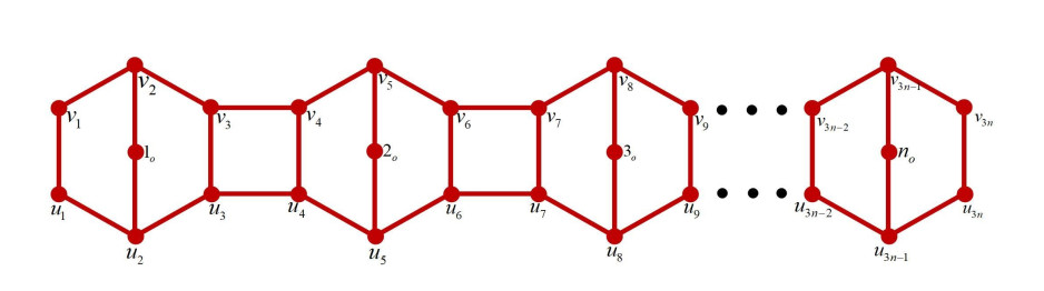
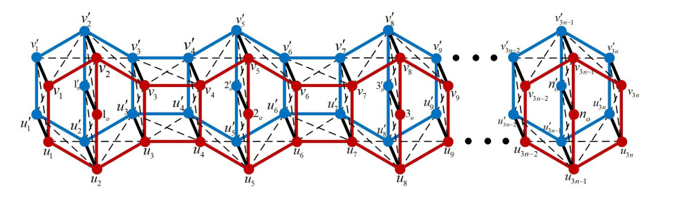
In this paper, we focus on the strong product of the pentagonal networks. Let $ R_{n} $ be a pentagonal network composed of $ 2n $ pentagons and $ n $ quadrilaterals. Let $ P_{n}^{2} $ denote the graph formed by the strong product of $ R_{n} $ and its copy $ R_{n}^{\prime} $. By utilizing the decomposition theorem of the normalized Laplacian characteristics polynomial, we characterize the explicit formula of the multiplicative degree-Kirchhoff index completely. Moreover, the complexity of $ P_{n}^{2} $ is determined.

| [1] | J. A. Bondy, U. S. R. Murty, Graph theory with applications, Macmillan Press Ltd., 1976. |
| [2] | F. R. K. Chung, Spectral graph theory, American Mathematical Society, 1997. |
| [3] |
H. Wiener, Structural determination of paraffin boiling points, J. Amer. Chem. Soc., 69 (1947), 17–20. https://doi.org/10.1021/ja01193a005 doi: 10.1021/ja01193a005

|
| [4] | A. Dobrynin, Branchings in trees and the calculation of the Wiener index of a tree, MATCH Commun. Math. Comput. Chem., 41 (2000), 119–134. |
| [5] |
A. A. Dobrynin, R. Entringer, I. Gutman, Wiener index of trees: theory and applications, Acta Appl. Math., 66 (2001), 211–249. https://doi.org/10.1023/A:1010767517079 doi: 10.1023/A:1010767517079
|
| [6] |
A. A. Dobrynin, I. Gutman, S. Klavžar, P. Žigert, Wiener index of hexagonal systems, Acta Appl. Math., 72 (2002), 247–294. https://doi.org/10.1023/A:1016290123303 doi: 10.1023/A:1016290123303
|
| [7] | F. Zhang, H. Li, Calculating Wiener numbers of molecular graphs with symmetry, MATCH Commun. Math. Comput. Chem., 35 (1997), 213–226. |
| [8] |
I. Gutman, S. Li, W. Wei, Cacti with $n$-vertices and $t$ cycles having extremal Wiener index, Discrete Appl. Math., 232 (2017), 189–200. https://doi.org/10.1016/j.dam.2017.07.023 doi: 10.1016/j.dam.2017.07.023
|
| [9] |
M. Knor, R. Škrekovski, A. Tepeh, Orientations of graphs with maximum Wiener index, Discrete Appl. Math., 211 (2016), 121–129. https://doi.org/10.1016/j.dam.2016.04.015 doi: 10.1016/j.dam.2016.04.015
|
| [10] |
I. Gutman, Selected properties of the Schultz molecular topological index, J. Chem. Inf. Comput. Sci., 34 (1994), 1087–1089. https://doi.org/10.1021/ci00021a009 doi: 10.1021/ci00021a009
|
| [11] | D. J. Klein, Resistance-distance sum rules, Croat. Chem. Acta, 75 (2002), 633–649. |
| [12] | D. J. Klein, O. Ivanciuc, Graph cyclicity, excess conductance, and resistance deficit, J. Math. Chem., 30 (2001), 271–287. https://doi.org/10.1023/A: 1015119609980 |
| [13] |
H. Chen, F. Zhang, Resistance distance and the normalized Laplacian spectrum, Discrete Appl. Math., 155 (2007), 654–661. https://doi.org/10.1016/j.dam.2006.09.008 doi: 10.1016/j.dam.2006.09.008
|
| [14] |
E. Bendito, A. Carmona, A. M. Encinas, J. M. Gesto, A formula for the Kirchhoff index, Int. J. Quantum Chem., 108 (2008), 1200–1206. https://doi.org/10.1002/qua.21588 doi: 10.1002/qua.21588
|
| [15] |
M. Bianchi, A. Cornaro, J. L. Palacios, A. Torriero, Bounds for the Kirchhoff index via majorization techniques, J. Math. Chem., 51 (2013), 569–587. https://doi.org/10.1007/s10910-012-0103-x doi: 10.1007/s10910-012-0103-x
|
| [16] |
G. P. Clemente, A. Cornaro, New bounds for the sum of powers of normalized Laplacian eigenvalues of graphs, Ars Math. Contemp., 11 (2016), 403–413. https://doi.org/10.26493/1855-3974.845.1B6 doi: 10.26493/1855-3974.845.1B6
|
| [17] | G. P. Clemente, A. Cornaro, Computing lower bounds for the Kirchhoff index via majorization techniques, MATCH Commun. Math. Comput. Chem., 73 (2015), 175–193. |
| [18] | J. L. Palacios, Closed-form formulas for Kirchhoff index, Int. J. Quantum Chem., 81 (2001), 135–140. |
| [19] |
J. L. Palacios, J. M. Renom, Another look at the degree-Kirchhoff index, Int. J. Quantum Chem., 111 (2011), 3453–3455. https://doi.org/10.1002/qua.22725 doi: 10.1002/qua.22725
|
| [20] |
W. Wang, D. Yang, Y. Luo, The Laplacian polynomial and Kirchhoff index of graphs derived from regular graphs, Discrete Appl. Math., 161 (2013), 3063–3071. https://doi.org/10.1016/j.dam.2013.06.010 doi: 10.1016/j.dam.2013.06.010
|
| [21] |
Y. Yang, H. Zhang, D. J. Klein, New Nordhaus-Gaddum-type results for the Kirchhoff index, J. Math. Chem., 49 (2011), 1587–1598. https://doi.org/10.1007/s10910-011-9845-0 doi: 10.1007/s10910-011-9845-0
|
| [22] |
H. Zhang, Y. Yang, C. Li, Kirchhoff index of composite graphs, Discrete Appl. Math., 157 (2009), 2918–2927. https://doi.org/10.1016/j.dam.2009.03.007 doi: 10.1016/j.dam.2009.03.007
|
| [23] |
B. Zhou, N. Trinajstić, On resistance-distance and Kirchhoff index, J. Math. Chem., 46 (2009), 283–289. https://doi.org/10.1007/s10910-008-9459-3 doi: 10.1007/s10910-008-9459-3
|
| [24] |
J. Huang, S. Li, X. Li, The normalized Laplacians degree-Kirchhoff index and spanning trees of the linear polyomino chains, Appl. Math. Comput., 289 (2016), 324–334. https://doi.org/10.1016/j.amc.2016.05.024 doi: 10.1016/j.amc.2016.05.024
|
| [25] |
Y. Pan, C. Liu, J. Li, Kirchhoff indices and numbers of spanning trees of molecular graphs derived from linear crossed polyomino chain, Polycyclic Aromat. Compd., 42 (2022), 218–225. https://doi.org/10.1080/10406638.2020.1725898 doi: 10.1080/10406638.2020.1725898
|
| [26] |
J. Liu, J. Zhao, Z. Zhu, On the number of spanning trees and normalized Laplacian of linear octagonal-quadrilateral networks, Int. J. Quantum Chem., 119 (2019), e25971. https://doi.org/10.1002/qua.25971 doi: 10.1002/qua.25971
|
| [27] |
L. Pavlović, I. Gutman, ChemInform abstract: Wiener numbers of phenylenes: an exact result, Chem. Inf., 28 (1997), 355–358. https://doi.org/10.1002/chin.199727271 doi: 10.1002/chin.199727271
|
| [28] | A. Chen, F. Zhang, Wiener index and perfect matchings in random phenylene chains, MATCH Commun. Math. Comput. Chem., 61 (2009), 623–630. |
| [29] |
J. Liu, Q. Zheng, Z. Cai, S. Hayat, On the Laplacians and normalized Laplacians for graph transformation with respect to the dicyclobutadieno derivative of [$n$] phenylenes, Polycyclic Aromat. Compd., 42 (2022), 1413–1434. https://doi.org/10.1080/10406638.2020.1781209 doi: 10.1080/10406638.2020.1781209
|
| [30] | X. He, The normalized Laplacian, degree-Kirchhoff index and spanning trees of graphs derived from the strong prism of linear polyomino chain, arXiv, 2020. https://doi.org/10.48550/arXiv.2008.07059 |
| [31] |
Z. Li, Z. Xie, J. Li, Y. Pan, Resistance distance-based graph invariants and spanning trees of graphs derived from the strong prism of a star, Appl. Math. Comput., 382 (2020), 125335. https://doi.org/10.1016/j.amc.2020.125335 doi: 10.1016/j.amc.2020.125335
|
| [32] |
J. Liu, J. Gu, Computing and analyzing the normalized Laplacian spectrum and spanning tree of the strong prism of the dicyclobutadieno derivative of linear phenylenes, Int. J. Quantum Chem., 122 (2022), e26972. https://doi.org/10.1002/QUA.26972 doi: 10.1002/QUA.26972
|
| [33] |
U. Ali, Y. Ahmad, S. Xu, X. Pan, On normalized Laplacian, degree-Kirchhoff index of the strong prism of generalized phenylenes, Polycyclic Aromat. Compd., 42 (2022), 6215–6232. https://doi.org/10.1080/10406638.2021.1977351 doi: 10.1080/10406638.2021.1977351
|
| [34] |
Y. Pan, J. Li, Kirchhoff index, multiplicative degree-Kirchhoff index and spanning trees of the linear crossed hexagonal chains, Int. J. Quantum Chem., 118 (2018), e25787. https://doi.org/10.1002/qua.25787 doi: 10.1002/qua.25787
|
| [35] |
Y. Yang, T. Yu, Graph theory of viscoelasticities for polymers with starshaped, multiple-ring and cyclic multiple-ring molecules, Die Makromol. Chem., 186 (1985), 609–631. https://doi.org/10.1002/macp.1985.021860315 doi: 10.1002/macp.1985.021860315
|
Figures(2)

Jia-Bao Liu, Kang Wang. The multiplicative degree-Kirchhoff index and complexity of a class of linear networks[J]. AIMS Mathematics, 2024, 9(3): 7111-7130. doi: 10.3934/math.2024347


 DownLoad: