Analyzing the impact of quantum computing on IoT security using computational based data analytics techniques

Wael Alosaimi; Abdullah Alharbi; Hashem Alyami; Bader Alouffi; Ahmed Almulihi; Mohd Nadeem; Rajeev Kumar; Alka Agrawal; Wael Alosaimi; Abdullah Alharbi; Hashem Alyami; Bader Alouffi; Ahmed Almulihi; Mohd Nadeem; Rajeev Kumar; Alka Agrawal

doi:10.3934/math.2024342

AIMS Mathematics

2024, Volume 9, Issue 3: 7017-7039. doi: 10.3934/math.2024342

Previous Article Next Article

Research article Special Issues

Analyzing the impact of quantum computing on IoT security using computational based data analytics techniques

1.
Department of Information Technology, College of Computers and Information Technology, Taif University, P.O. Box 11099, Taif 21944, Saudi Arabia
2.
Department of Computer Science, College of Computers and Information Technology, Taif University, P. O. Box 11099, Taif 21944, Saudi Arabia
3.
School of Computer Application, Babu Banarasi Das University, Lucknow, UP, India 226028
4.
Centre for Innovation and Technology, Administrative Staff College of India, Hyderabad, Telangana, India 500082
5.
Department of Information Technology, Babasaheb Bhimrao Ambedkar University, Lucknow, UP, India 226025

Received: 05 December 2023 Revised: 15 January 2024 Accepted: 23 January 2024 Published: 19 February 2024
MSC : 03B52, 94D05, 94D10

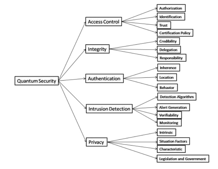
The Internet of Things (IoT) market is experiencing exponential growth, with projections increasing from 15 billion dollars to an estimated 75 billion dollars by 2025. Quantum computing has emerged as a key enabler for managing the rapid expansion of IoT technology, serving as the foundation for quantum computing support. However, the adoption of quantum computing also introduces numerous privacy and security challenges. We delve into the critical realm of quantum-level security within a typical quantum IoT. To achieve this objective, we identified and precisely analyzed security attributes at various levels integral to quantum computing. A hierarchical tree of quantum computing security attributes was envisioned, providing a structured approach for systematic and efficient security considerations. To assess the impact of security on the quantum-IoT landscape, we employed a unified computational model based on Multi-Criteria Decision-Making (MCDM), incorporating the Analytical Hierarchy Process (AHP) and the Technique for Ordering Preferences by Similarity to Ideal Solutions (TOPSIS) within a fuzzy environment. Fuzzy sets were used to provide practical solutions that can accommodate the nuances of diverse and ambiguous opinions, ultimately yielding precise alternatives and factors. The projected undertaking was poised to empower practitioners in the quantum-IoT realm by aiding in the identification, selection, and prioritization of optimal security factors through the lens of quantum computing.
- quantum security,
- quantum computing,
- internet of things,
- fuzzy decision making
Citation: Wael Alosaimi, Abdullah Alharbi, Hashem Alyami, Bader Alouffi, Ahmed Almulihi, Mohd Nadeem, Rajeev Kumar, Alka Agrawal. Analyzing the impact of quantum computing on IoT security using computational based data analytics techniques[J]. AIMS Mathematics, 2024, 9(3): 7017-7039. doi: 10.3934/math.2024342

Related Papers:

Abstract

The Internet of Things (IoT) market is experiencing exponential growth, with projections increasing from 15 billion dollars to an estimated 75 billion dollars by 2025. Quantum computing has emerged as a key enabler for managing the rapid expansion of IoT technology, serving as the foundation for quantum computing support. However, the adoption of quantum computing also introduces numerous privacy and security challenges. We delve into the critical realm of quantum-level security within a typical quantum IoT. To achieve this objective, we identified and precisely analyzed security attributes at various levels integral to quantum computing. A hierarchical tree of quantum computing security attributes was envisioned, providing a structured approach for systematic and efficient security considerations. To assess the impact of security on the quantum-IoT landscape, we employed a unified computational model based on Multi-Criteria Decision-Making (MCDM), incorporating the Analytical Hierarchy Process (AHP) and the Technique for Ordering Preferences by Similarity to Ideal Solutions (TOPSIS) within a fuzzy environment. Fuzzy sets were used to provide practical solutions that can accommodate the nuances of diverse and ambiguous opinions, ultimately yielding precise alternatives and factors. The projected undertaking was poised to empower practitioners in the quantum-IoT realm by aiding in the identification, selection, and prioritization of optimal security factors through the lens of quantum computing.

References

[1]	R. Kaewpuang, M. Xu, D. Niyato, H. Yu, Z. Xiong, J. Kang, Stochastic Qubit Resource Allocation for Quantum Cloud Computing, NOMS 2023-2023 IEEE/IFIP Network Operations and Management Symposium, Miami, FL, USA, 2023, 1–5. https://doi.org/10.1109/NOMS56928.2023.10154430
[2]	H. Alyami, M. Nadeem, A. Alharbi, W. Alosaimi, M. T. J. Ansari, D. Pandey, et al., The evaluation of software security through quantum computing techniques: A durability perspective, Appl. Sci., 11 (2021), 11784. https://doi.org/10.3390/app112411784 doi: 10.3390/app112411784
[3]	S. H. Almotiri, M. Nadeem, M. A. Al Ghamdi, R. A. Khan, Analytic review of healthcare software by using quantum computing security techniques, IJFIS, 23 (2023), 336–352. https://doi.org/10.5391/IJFIS.2023.23.3.336 doi: 10.5391/IJFIS.2023.23.3.336
[4]	D. Koo, Y. Shin, J. Yun, J. Hur, A Hybrid Deduplication for Secure and Efficient Data Outsourcing in Fog Computing 2016 IEEE International Conference on Cloud Computing Technology and Science (CloudCom), Luxembourg, Luxembourg, 2016,285–293. https://doi.org/10.1109/CloudCom.2016.0054
[5]	L. Zhao, Privacy-preserving distributed analytics in Fog-Enabled IoT systems, Sensors, 20 (2020), 6153. https://doi.org/10.3390/s20216153 doi: 10.3390/s20216153
[6]	K. Xue, J. Hong, Y. Ma, D. S. L. Wei, P. Hong, N. Yu, Fog-Aided verifiable privacy preserving access control for latency-sensitive data sharing in vehicular cloud computing, IEEE Network, 32 (2018), 7–13. https://doi.org/10.1109/MNET.2018.1700341 doi: 10.1109/MNET.2018.1700341
[7]	H. Wang, Z. Wang, J. D. Ferrer, Anonymous and secure aggregation scheme in fog-based public cloud computing, Future Gener. Comp. Sy., 78 (2018), 712–719. https://doi.org/10.1016/j.future.2017.02.032 doi: 10.1016/j.future.2017.02.032
[8]	J. Zhao, F. Huang, L. Liao, Q. Zhang, Blockchain-based trust management model for vehicular Ad Hoc networks, IEEE Internet Things, 1, (2023), 1–10. https://doi.org/10.1109/JIOT.2023.3318597 doi: 10.1109/JIOT.2023.3318597
[9]	J. Zhao, H. Hu, F. Huang, Y. Guo, L. Liao, Authentication technology in internet of things and privacy security issues in typical application scenarios, Electronics, 12 (2023), 1812. https://doi.org/10.3390/electronics12081812 doi: 10.3390/electronics12081812
[10]	L. Liao, J. Zhao, H. Hu, X. Sun, Secure and efficient message authentication scheme for 6G-Enabled VANETs, Electronics, 11 (2022), 2385. https://doi.org/10.3390/electronics11152385 doi: 10.3390/electronics11152385
[11]	R. Lu, K. Heung, A. H. Lashkari, A. A. Ghorbani, A lightweight privacy-preserving data aggregation scheme for fog computing-enhanced IoT, IEEE Access, 5 (2017), 3302–3312. https://doi.org/10.1109/ACCESS.2017.2677520 doi: 10.1109/ACCESS.2017.2677520
[12]	A. Rauf, R. A. Shaikh, A. Shah, Security and privacy for IoT and fog computing paradigm, 2018 15th Learning and Technology Conference (L & T), Jeddah, Saudi Arabia, 2018, 96–101. https://doi.org/10.1109/LT.2018.8368491
[13]	T. D. Dang, D. Hoang, A data protection model for fog computing, 2017 Second International Conference on Fog and Mobile Edge Computing (FMEC), Valencia, Spain, 2017, 32–38. https://doi.org/10.1109/FMEC.2017.7946404
[14]	P. Zhang, Z. Chen, J. K. Liu, K. Liang, H. Liu, An efficient access control scheme with outsourcing capability and attribute update for fog computing, Future Gener. Comp. Sy., 78 (2018), 753–762. https://doi.org/10.1016/j.future.2016.12.015 doi: 10.1016/j.future.2016.12.015
[15]	K. Vohra, M. Dave, Multi-authority attribute-based data access control in fog computing, Procedia Comput. Sci., 132 (2018), 1449–1457. https://doi.org/10.1016/j.procs.2018.05.078 doi: 10.1016/j.procs.2018.05.078
[16]	M. Xiao, J. Zhou, X. Liu, M. Jiang, A hybrid scheme for Fine-Grained search and access authorization in fog computing environment, Sensors, 17 (2017), 1423. https://doi.org/10.3390/s17061423 doi: 10.3390/s17061423
[17]	I. Stojmenovic, S. Wen, X. Huang, H. Luan, An overview of Fog computing and its security issues, Concurr. Comput. Pract. Exp., 28 (2016), 2991–3005. https://doi.org/10.1002/cpe.3485 doi: 10.1002/cpe.3485
[18]	S. Homayoun, A. Dehghantanha, M. Ahmadzadeh, S. Hashemi, R. Khayami, K. Raymond Choo, DRTHIS: Deep ransomware threat hunting and intelligence system at the fog layer, Future Gener. Comp. Sy., 90 (2019), 94–104. https://doi.org/10.1016/j.future.2018.07.045 doi: 10.1016/j.future.2018.07.045
[19]	K. Sahu, F. A. Alzahrani, R. K. Srivastava, R. Kumar, Hesitant fuzzy sets based symmetrical model of decision-making for estimating the durability of web application, Symmetry, 12 (2020), 1770. https://doi.org/10.3390/sym12111770 doi: 10.3390/sym12111770
[20]	S. A. Khan, M. Alenezi, A. Agrawal, R. Kumar, R. A. Khan, Evaluating performance of software durability through an integrated fuzzy-based symmetrical method of ANP and TOPSIS, Symmetry, 12 (2020), 493. https://doi.org/10.3390/sym12040493 doi: 10.3390/sym12040493
[21]	P. C. Pathak, M. Nadeem, S. A. Ansar, Security assessment of operating system by using decision making algorithms, Int. J. Inf. Tecnol., 9 (2024), 1–11. https://doi.org/10.1007/s41870-023-01706-9 doi: 10.1007/s41870-023-01706-9
[22]	B. A. Mozzaquatro, C. Agostinho, D Goncalves, J. Martins, R. Jardim-Goncalves, An ontology-based cybersecurity framework for the internet of things, Sensors, 18 (2018), 3053. https://doi.org/10.3390/s18093053 doi: 10.3390/s18093053
[23]	J. Kaur, A. Agrawal, R. A. Khan, Security assessment in Foggy Era through analytical hierarchy process, 2020 11th International Conference on Computing, Communication and Networking Technologies (ICCCNT), Kharagpur, India, 2020, 1–6. https://doi.org/10.1109/ICCCNT49239.2020.9225308
[24]	R. Verma, S. Chandra, Interval-valued intuitionistic fuzzy-analytic hierarchy process for evaluating the impact of security attributes in fog-based internet of things paradigm, Comput. Commun., 175 (2021), 35–46. https://doi.org/10.1016/j.comcom.2021.04.019 doi: 10.1016/j.comcom.2021.04.019
[25]	J. Kaur, A. Agrawal, R. A. Khan, Security Issues in Fog Environment: A Systematic Literature Review, Int. J. Wireless Inf. Networks, 27 (2020), 467–483. https://doi.org/10.1007/s10776-020-00491-7 doi: 10.1007/s10776-020-00491-7
[26]	J. Kaur, A. I. Khan, Y. B. Abushark, M. M. Alam, S. A. Khan, A. Agrawal, et al., Security risk assessment of healthcare web application through adaptive neuro-fuzzy inference system: A design perspective, Risk Manag. Healthc. P., 13 (2020), 1–21. https://doi.org/10.2147/RMHP.S233706 doi: 10.2147/RMHP.S233706
[27]	J. Kaur, R. Verma, N. Alharbe, A. Agrawal, R. A. Khan, Importance of fog computing in healthcare 4.0, Signals Commun. Technol., 4 (2021) 79–101. https://doi.org/10.1007/978-3-030-46197-3_4 doi: 10.1007/978-3-030-46197-3_4
[28]	R. Verma, S. Chandra, A systematic survey on fog steered IoT: Architecture, prevalent threats and trust models, Int. J. Wireless Inf. Networks, 28 (2021), 116–133. https://doi.org/10.1007/s10776-020-00499-z doi: 10.1007/s10776-020-00499-z
[29]	S. A. Khan, M. Nadeem, A. Agrawal, R. A. Khan, R. Kumar, Quantitative analysis of software security through fuzzy PROMETHEE-Ⅱ methodology: A design perspective, IJMECS, 13 (2021), 30–41. https://doi.org/10.5815/ijmecs.2021.06.04 doi: 10.5815/ijmecs.2021.06.04
[30]	R. Verma, S. Chandra, Security and privacy issues in fog driven IoT environment, Int. J. Comput. Sci. Eng., 7 (2019), 367–370. https://doi.org/10.26438/ijcse/v7i5.367370 doi: 10.26438/ijcse/v7i5.367370
[31]	R. Verma, S. Chandra, A Fuzzy AHP approach for ranking security attributes in Fog-IoT environment, 2020 11th International Conference on Computing, Communication and Networking Technologies (ICCCNT), Kharagpur, India, 2020, 1–5. https://doi.org/10.1109/ICCCNT49239.2020.9225513
[32]	M. Ahmad, J. F. Al-Amri, A. F. Subahi, S. Khatri, A. H. Seh, M. Nadeem, et al., Healthcare device security assessment through computational methodology, Comput. Syst. Sci. Eng., 41 (2022), 811–828. https://doi.org/10.32604/csse.2022.020097 doi: 10.32604/csse.2022.020097
[33]	A. Attaallah, M. Ahmad, M. T. J. Ansari, A. K. Pandey, R. Kumar, R. A. Khan, et al., Device security assessment of internet of healthcare things, Intell. Autom. Soft Co., 27 (2021), 593–603. https://doi.org/10.32604/iasc.2021.015092 doi: 10.32604/iasc.2021.015092
[34]	M. T. J. Ansari, A. Baz, H. Alhakami et al., P-STORE: Extension of STORE Methodology to Elicit Privacy Requirements, Arab. J. Sci. Eng., 46 (2021), 8287–8310. https://doi.org/10.1007/s13369-021-05476-z doi: 10.1007/s13369-021-05476-z
[35]	F. A. Alzahrani, M. Ahmad, M. Nadeem, R. Kumar, R. A. Khan, Integrity assessment of medical devices for improving hospital services, Comput. Mater. Con., 67 (2021), 3619–3633. https://doi.org/10.32604/cmc.2021.014869 doi: 10.32604/cmc.2021.014869
[36]	K. Sahu, F. A. Alzahrani, R. K. Srivastava, R. Kumar, Evaluating the impact of prediction techniques: software reliability perspective, Comput. Mater. Con., 67 (2021), 1471–1488. https://doi.org/10.32604/cmc.2021.014868 doi: 10.32604/cmc.2021.014868
[37]	R. Kumar, M. T. J. Ansari, A. Baz, H. Alhakami, A. Agrawal, et al., A multi-perspective benchmarking framework for estimating usable-security of hospital management system software based on fuzzy logic, ANP and TOPSIS methods, KSⅡ T. Internet Inf., 15 (2021), 240–263. https://doi.org/10.3837/tiis.2021.01.014 doi: 10.3837/tiis.2021.01.014
[38]	F. A. Al-Zahrani, Evaluating the Usable-Security of healthcare software through unified technique of fuzzy logic, ANP and TOPSIS, IEEE Access, 8 (2020), 109905–109916. https://doi.org/10.1109/ACCESS.2020.3001996 doi: 10.1109/ACCESS.2020.3001996
[39]	M. T. J. Ansari, D. Pandey, M. Alenezi, STORE: security threat oriented requirements engineering methodology, J. King Saud Univ.-Com., 34 (2022), 191–203. https://doi.org/10.1016/j.jksuci.2018.12.005 doi: 10.1016/j.jksuci.2018.12.005
[40]	W. Alosaimi, A. Alharbi, H. Alyami, M. Ahmad, A. K. Pandey, R. Kumar, et al., Impact of tools and techniques for securing consultancy services, Comput. Syst. Sci. Eng., 37 (2021), 347–360. https://doi.org/10.32604/csse.2021.015284 doi: 10.32604/csse.2021.015284
[41]	K. Sahu, R. K. Srivastava, Predicting software bugs of newly and large datasets through a unified neuro-fuzzy approach: Reliability perspective, Adv. Math. Sci. J., 10 (2021), 543–555. https://doi.org/10.37418/amsj.10.1.54 doi: 10.37418/amsj.10.1.54

Reader Comments

Your name:*

Email:*
© 2024 the Author(s), licensee AIMS Press. This is an open access article distributed under the terms of the Creative Commons Attribution License (http://creativecommons.org/licenses/by/4.0)