Numerical investigation of convergence in the $ L^{\infty} $ norm for modified SGFEM applied to elliptic interface problems

Pengfei Zhu; Kai Liu; Pengfei Zhu; Kai Liu

doi:10.3934/math.20241507

AIMS Mathematics

2024, Volume 9, Issue 11: 31252-31273. doi: 10.3934/math.20241507

Previous Article Next Article

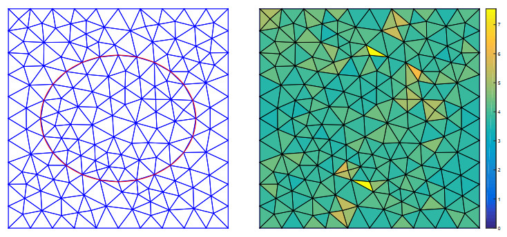
Research article Special Issues

Numerical investigation of convergence in the $L^{\infty}$ norm for modified SGFEM applied to elliptic interface problems

Pengfei Zhu ^{1
,
,},
Kai Liu ²

1.
School of Computer and Information Engineering, Guizhou University of Commerce, Guiyang 550014, China
2.
School of Science, East China University of Technology, Nanchang 330013, China

Received: 23 August 2024 Revised: 11 October 2024 Accepted: 21 October 2024 Published: 04 November 2024
MSC : 65N12, 65N30

Convergence in the $L^{\infty}$ norm is a very important consideration in numerical simulations of interface problems. In this paper, a modified stable generalized finite element method (SGFEM) was proposed for solving the second-order elliptic interface problem in the two-dimensional bounded and convex domain. The proposed SGFEM uses a one-side enrichment function. There is no stability term in the weak form of the model problem, and it is a conforming finite element method. Moreover, it is applicable to any smooth interface, regardless of its concavity or shape. Several nontrivial examples illustrate the excellent properties of the proposed SGFEM, including its convergence in both the $L^2$ and $L^{\infty}$ norms, as well as its stability and robustness.

Keywords:

Citation: Pengfei Zhu, Kai Liu. Numerical investigation of convergence in the $L^{\infty}$ norm for modified SGFEM applied to elliptic interface problems[J]. AIMS Mathematics, 2024, 9(11): 31252-31273. doi: 10.3934/math.20241507

Related Papers:

[1]	Yasmina Khiar, Esmeralda Mainar, Eduardo Royo-Amondarain, Beatriz Rubio . High relative accuracy for a Newton form of bivariate interpolation problems. AIMS Mathematics, 2025, 10(2): 3836-3847. doi: 10.3934/math.2025178
[2]	Chih-Hung Chang, Ya-Chu Yang, Ferhat Şah . Reversibility of linear cellular automata with intermediate boundary condition. AIMS Mathematics, 2024, 9(3): 7645-7661. doi: 10.3934/math.2024371
[3]	Yongge Tian . Miscellaneous reverse order laws and their equivalent facts for generalized inverses of a triple matrix product. AIMS Mathematics, 2021, 6(12): 13845-13886. doi: 10.3934/math.2021803
[4]	Yang Chen, Kezheng Zuo, Zhimei Fu . New characterizations of the generalized Moore-Penrose inverse of matrices. AIMS Mathematics, 2022, 7(3): 4359-4375. doi: 10.3934/math.2022242
[5]	Pattrawut Chansangiam, Arnon Ploymukda . Riccati equation and metric geometric means of positive semidefinite matrices involving semi-tensor products. AIMS Mathematics, 2023, 8(10): 23519-23533. doi: 10.3934/math.20231195
[6]	Zongcheng Li, Jin Li . Linear barycentric rational collocation method for solving a class of generalized Boussinesq equations. AIMS Mathematics, 2023, 8(8): 18141-18162. doi: 10.3934/math.2023921
[7]	Maolin Cheng, Bin Liu . A novel method for calculating the contribution rates of economic growth factors. AIMS Mathematics, 2023, 8(8): 18339-18353. doi: 10.3934/math.2023932
[8]	Junsheng Zhang, Lihua Hao, Tengyun Jiao, Lusong Que, Mingquan Wang . Mathematical morphology approach to internal defect analysis of A356 aluminum alloy wheel hubs. AIMS Mathematics, 2020, 5(4): 3256-3273. doi: 10.3934/math.2020209
[9]	Sizhong Zhou, Quanru Pan . The existence of subdigraphs with orthogonal factorizations in digraphs. AIMS Mathematics, 2021, 6(2): 1223-1233. doi: 10.3934/math.2021075
[10]	Salman Zeb, Muhammad Yousaf, Aziz Khan, Bahaaeldin Abdalla, Thabet Abdeljawad . Updating $QR$ factorization technique for solution of saddle point problems. AIMS Mathematics, 2023, 8(1): 1672-1681. doi: 10.3934/math.2023085

Abstract

1. Introduction

Throughout this article, ${\mathbb C}^{m \times n}$ denotes the collection of all $m \times n$ matrices over the field of complex numbers, $A^{\ast}$ denotes the conjugate transpose of $A \in {\mathbb C}^{m \times n}$ , $r(A)$ denotes the rank of $A \in {\mathbb C}^{m \times n}$ , ${\mathscr R}(A)$ denotes the range of $A \in {\mathbb C}^{m \times n}$ , $I_m$ denotes the identity matrix of order $m$ , and $[\, A, \, B\, ]$ denotes a row block matrix consisting of $A\in {\mathbb C}^{m \times n}$ and $B\in {\mathbb C}^{m \times p}$ . The Moore-Penrose generalized inverse of $A \in {\mathbb C}^{m \times n}$ , denoted by $A^{\dagger}$ , is the unique matrix $X \in {\mathbb C}^{n \times m}$ satisfying the four Penrose equations

${\rm (1)} \ AXA = A, \ \ {\rm (2)} \ XAX = X, \ \ {\rm (3)} \ (AX)^{*} = AX, \ \ {\rm (4)} \ (XA)^{*} = XA.$

Further, we denote by

$\begin{align} P_A = AA^{\dagger}, \ \ E_{A} = I_m - AA^{\dagger} \end{align}$

(1.1)

the two orthogonal projectors induced from $A\in {\mathbb C}^{m \times n}$ . For more detailed information regarding generalized inverses of matrices, we refer the reader to ^[2,3,4].

Recall that the well-known Kronecker product of any two matrices $A = (a_{ij}) \in {\mathbb C}^{m \times n}$ and $B = (b_{ij}) \in {\mathbb C}^{p \times q}$ is defined to be

$A \otimes B = (a_{ij}B) = \begin{bmatrix} a_{11}B & a_{12}B & \cdots & a_{1n}B \\ a_{21}B & a_{22}B & \cdots & a_{2n}B \\ \vdots & \vdots & \ddots & \vdots \\ a_{m1}B & a_{m2}B & \cdots & a_{mn}B \end{bmatrix} \in {\mathbb C}^{mp \times nq}.$

The Kronecker product, named after German mathematician Leopold Kronecker, was classified to be a special kind of matrix operation, which has been regarded as an important matrix operation and mathematical technique. This product has wide applications in system theory, matrix calculus, matrix equations, system identification and more (cf. ^{[1,5,6,7,8,9,10,11,12,13,14,16,18,19,20,21,23,24,25,27,28,33,34]}). It has been known that the matrices operations based on Kronecker products have a series of rich and good structures and properties, and thus they have many significant applications in the research areas of both theoretical and applied mathematics. In fact, mathematicians established a variety of useful formulas and facts related to the products and used them to deal with various concrete scientific computing problems. Specifically, the basic facts on Kronecker products of matrices in the following lemma were highly appraised and recognized (cf. ^{[15,17,21,32,34]}).

Fact 1.1. Let $A \in {\mathbb C}^{m \times n},$ $B \in {\mathbb C}^{p \times q},$ $C \in {\mathbb C}^{n \times s},$ and $D\in {\mathbb C}^{q \times t}.$ Then $,$ the following equalities hold $:$

$\begin{align} & \ \ \ \ \ \ (A \otimes B)(C \otimes D) = (AC) \otimes (BD), \end{align}$

(1.2)

$\begin{align} & (A \otimes B)^{*} = A^{*} \otimes B^{*}, \ \ \ (A \otimes B)^{\dagger} = A^{\dagger} \otimes B^{\dagger}, \end{align}$

(1.3)

$\begin{align} & P_{A\otimes B} = P_{A} \otimes P_{B}, \ \ \ \ \ \ r(A \otimes B) = r(A)r(B). \end{align}$

(1.4)

In addition, the Kronecker product of matrices has a rich variety of algebraic operation properties. For example, one of the most important features is that the product $A_1 \otimes A_2$ can be factorized as certain ordinary products of matrices:

$\begin{align} A_1 \otimes A_2 = (A_1 \otimes I_{m_2})(I_{n_1} \otimes A_2) = (I_{m_1} \otimes A_2)(A_1 \otimes I_{n_2}) \end{align}$

(1.5)

for any $A_1 \in {\mathbb C}^{m_1 \times n_1}$ and $A_2 \in {\mathbb C}^{m_2 \times n_2}$ , and the triple Kronecker product $A_1 \otimes A_2 \otimes A_3$ can be written as

$\begin{align} A_1 \otimes A_2 \otimes A_3 & = (A_1\otimes I_{m_2} \otimes I_{m_3})(I_{n_1} \otimes A_2 \otimes I_{m_3})(I_{n_1} \otimes I_{n_2} \otimes A_3) , \end{align}$

(1.6)

$\begin{align} A_1 \otimes A_2 \otimes A_3 & = (I_{n_1} \otimes A_2 \otimes I_{m_3})(I_{n_1}(I_{n_1} \otimes I_{n_2} \otimes A_3) (A_1\otimes I_{m_2} \otimes I_{m_3}), \end{align}$

(1.7)

$\begin{align} A_1 \otimes A_2 \otimes A_3 & = (I_{m_1} \otimes I_{m_2} \otimes A_3)(A_1 \otimes I_{n_2} \otimes I_{n_3})(I_{m_1} \otimes A_2 \otimes I_{n_3}) \end{align}$

(1.8)

for any $A_1 \in {\mathbb C}^{m_1 \times n_1}$ , $A_2 \in {\mathbb C}^{m_2 \times n_2}$ and $A_3 \in {\mathbb C}^{m_3 \times n_3}$ , where the five matrices in the parentheses on the right hand sides of (1.5)–(1.8) are usually called the dilation expressions of the given three matrices $A_1$ , $A_2$ and $A_3$ , and the four equalities in (1.5)–(1.8) are called the dilation factorizations of the Kronecker products $A_1 \otimes A_2$ and $A_1 \otimes A_2 \otimes A_3$ , respectively. A common feature of the four matrix equalities in (1.5)–(1.8) is that they factorize Kronecker products of any two or three matrices into certain ordinary products of the dilation expressions of $A_1$ , $A_2$ and $A_3$ . Particularly, a noticeable fact we have to point out is that the nine dilation expressions of matrices in (1.5)–(1.8) commute each other by the well-known mixed-product property in (1.2) when $A_1$ , $A_2$ and $A_3$ are all square matrices. It can further be imagined that there exists proper extension of the dilation factorizations to Kronecker products of multiple matrices. Although the dilation factorizations in (1.5)–(1.8) seem to be technically trivial in form, they can help deal with theoretical and computational issues regarding Kronecker products of two or three matrices through the ordinary addition and multiplication operations of matrices.

In this article, we provide a new analysis of performances and properties of Kronecker products of matrices, as well as present a wide range of novel and explicit facts and results through the dilation factorizations described in (1.5)–(1.8) for the purpose of obtaining a deeper understanding and grasping of Kronecker products of matrices, including a number of analytical formulas for calculating ranks, dimensions, orthogonal projectors, and ranges of the dilation expressions of matrices and their algebraic operations.

The remainder of article is organized as follows. In section two, we introduce some preliminary facts and results concerning ranks, ranges, and generalized inverses of matrices. In section three, we propose and prove a collection of useful equalities, inequalities, and formulas for calculating the ranks, dimensions, orthogonal projectors, and ranges associated with the Kronecker products $A_1 \otimes A_2$ and $A_1 \otimes A_2 \otimes A_3$ through the dilation expressions of $A_1$ , $A_2$ and $A_3$ and their operations. Conclusions and remarks are given in section four.

2. Some preliminaries

One of the remarkable applications of generalized inverses of matrices is to establish various exact and analytical expansion formulas for calculating the ranks of partitioned matrices. As convenient and skillful tools, these matrix rank formulas can be used to deal with a wide variety of theoretical and computational issues in matrix theory and its applications (cf. ^[22]). In this section, we present a mixture of commonly used formulas and facts in relation to ranks of matrices and their consequences about the commutativity of two orthogonal projectors, which we shall use as analytical tools to approach miscellaneous formulas related to Kronecker products of matrices.

Lemma 2.1. ^[22,29] Let $A \in {\mathbb C}^{m \times n}$ and $B \in {\mathbb C}^{ m \times k}.$ Then $,$ the following rank equalities

$\begin{align} & r[A, \, B] = r(A) + r(E_AB) = r(B) + r(E_BA), \end{align}$

(2.1)

$\begin{align} & r[A, \, B] = r(A) + r(B) - 2r(A^*B) + r[P_{A}P_{B}, \, P_{B}P_{A}], \end{align}$

(2.2)

$\begin{align} & r[A, \, B] = r(A) + r(B) - r(A^*B) + 2^{-1}r(P_AP_B - P_BP_A), \end{align}$

(2.3)

$\begin{align} & r[A, \, B] = r(A) + r(B) - r(A^*B) + r(P_{[A, \, B]} - P_A - P_B + P_AP_B) \end{align}$

(2.4)

hold $.$ Therefore $,$

$\begin{align} P_AP_B = P_BP_A &\Leftrightarrow P_{[A, \, B]} = P_A + P_B - P_AP_B \\ &\Leftrightarrow r(E_AB) = r(B) - r(A^*B) \\ & \Leftrightarrow r[A, \, B] = r(A) + r(B) - r(A^*B) \\ & \Leftrightarrow {\mathscr R}(P_{A}P_{B}) = {\mathscr R}(P_{B}P_{A}). \end{align}$

(2.5)

If $P_AP_B = P_BP_A,$ $P_AP_C = P_CP_A$ and $P_BP_C = P_CP_B,$ then

$\begin{align} P_{[A, \, B, \, C]} = P_A + P_B + P_C - P_AP_B - P_AP_C - P_BP_C + P_AP_BP_C. \end{align}$

(2.6)

Lemma 2.2. ^[30] Let $A, \, B$ and $C \in {\mathbb C}^{m \times m}$ be three idempotent matrices $.$ Then $,$ the following rank equality

$\begin{align} r[A, \, B, \, C] & = r(A) + r(B) + r(C) - r[AB, \, AC] - r[BA, \, BC] - r[CA, \, CB] \\ & \ \ \ + r[AB, \, AC, \, BA, \, BC, \, CA, \, CB] \end{align}$

(2.7)

holds $.$ As a special instance $,$ if $AB = BA,$ $AC = CA$ and $BC = CB,$ then

$\begin{align} r[A, \, B, \, C] & = r(A) + r(B) + r(C) - r[AB, \, AC] - r[BA, \, BC] - r[CA, \, CB] + r[AB, \, AC, \, BC]. \end{align}$

(2.8)

The formulas and facts in the above two lemmas belong to mathematical competencies and conceptions in ordinary linear algebra. Thus they can easily be understood and technically be utilized to establish and simplify matrix expressions and equalities consisting of matrices and their generalized inverses.

3. Main results

We first establish a group of formulas and facts associated with the orthogonal projectors, ranks, dimensions, and ranges of the matrix product in (1.5).

Theorem 3.1. Let $A_1 \in {\mathbb C}^{m_1 \times n_1}$ and $A_2 \in {\mathbb C}^{m_2 \times n_2},$ and denote by

$M_1 = A_1 \otimes I_{m_2}, \ \ M_2 = I_{m_1} \otimes A_2$

the two dilation expressions of $A_1$ and $A_2,$ respectively $.$ Then $,$ we have the following results $.$

${\rm (a)}$ The following orthogonal projector equalities hold $:$

$\begin{align} P_{A_1 \otimes A_2} = P_{M_1}P_{M_2} = P_{M_2}P_{M_1} = P_{A_1} \otimes P_{A_2}. \end{align}$

(3.1)

${\rm (b)}$ The following four rank equalities hold $:$

$\begin{align} r[A_1 \otimes I_{m_2}, \, I_{m_1} \otimes A_2] & = m_1m_2 - (m_1 - r(A_1))(m_2 - r(A_2)), \end{align}$

(3.2)

$\begin{align} r[A_1 \otimes I_{m_2}, \, I_{m_1} \otimes E_{A_2}] & = m_1m_2 - (m_1 - r(A_1))r(A_2), \end{align}$

(3.3)

$\begin{align} r[E_{A_1} \otimes I_{m_2}, \, I_{m_1} \otimes A_2] & = m_1m_2 - r(A_1)(m_2 - r(A_2)), \end{align}$

(3.4)

$\begin{align} r[E_{A_1} \otimes I_{m_2}, \, I_{m_1} \otimes E_{A_2}] & = m_1m_2 - r(A_1)r(A_2), \end{align}$

(3.5)

and the following five dimension equalities hold $:$

$\begin{align} \dim( {\mathscr R}(M_1)\cap {\mathscr R}(M_2)) & = r(M_1M_2) = r(A_1)r(A_2), \end{align}$

(3.6)

$\begin{align} \dim( {\mathscr R}(M_1)\cap {\mathscr R}^{\perp}(M_2)) & = r(M_1E_{M_2}) = r(A_1)(m_2 - r(A_2)), \end{align}$

(3.7)

$\begin{align} \dim( {\mathscr R}^{\perp}(M_1)\cap {\mathscr R}(M_2)) & = r(E_{M_1}M_2) = (m_1 - r(A_1))r(A_2), \end{align}$

(3.8)

$\begin{align} \dim( {\mathscr R}^{\perp}(M_1)\cap {\mathscr R}^{\perp}(M_2)) & = r(E_{M_1}E_{M_2}) = (m_1 - r(A_1))(m_2 - r(A_2)), \end{align}$

(3.9)

$\begin{align} &\dim( {\mathscr R}(M_1)\cap {\mathscr R}(M_2)) + \dim( {\mathscr R}(M_1)\cap {\mathscr R}^{\perp}(M_2)) + \dim( {\mathscr R}^{\perp}(M_1)\cap {\mathscr R}^{\perp}(M_2)) \\ & \ + \dim( {\mathscr R}^{\perp}(M_1)\cap {\mathscr R}^{\perp}(M_2)) = m_1m_2. \end{align}$

(3.10)

${\rm (c)}$ The following range equalities hold $:$

$\begin{align} {\mathscr R}(M_1)\cap {\mathscr R}(M_2) & = {\mathscr R}(M_1M_2) = {\mathscr R}(M_2M_1) = {\mathscr R}(A_1 \otimes A_2), \end{align}$

(3.11)

$\begin{align} {\mathscr R}(M_1)\cap {\mathscr R}^{\perp}(M_2) & = {\mathscr R}(M_1E_{M_2}) = {\mathscr R}(E_{M_2}M_1) = {\mathscr R}(A_1 \otimes E_{A_2}), \end{align}$

(3.12)

$\begin{align} {\mathscr R}^{\perp}(M_1)\cap {\mathscr R}(M_2) & = {\mathscr R}(E_{M_1}M_2) = {\mathscr R}(M_2E_{M_1}) = {\mathscr R}(E_{A_1} \otimes A_2), \end{align}$

(3.13)

$\begin{align} {\mathscr R}^{\perp}(M_1)\cap {\mathscr R}^{\perp}(M_2) & = {\mathscr R}(E_{M_1}E_{M_2}) = {\mathscr R}(E_{M_2}E_{M_1}) = {\mathscr R}(E_{A_1} \otimes E_{A_2}), \end{align}$

(3.14)

$\begin{align} & ( {\mathscr R}(M_1)\cap {\mathscr R}(M_2)) \oplus ( {\mathscr R}^{\perp}(M_1)\cap {\mathscr R}(M_2)) \oplus ( {\mathscr R}(M_1)\cap {\mathscr R}^{\perp}(M_2)) \oplus ( {\mathscr R}^{\perp}(M_1)\cap {\mathscr R}^{\perp}(M_2)) \\ & = {\mathbb C}^{m_1m_2}. \end{align}$

(3.15)

${\rm (d)}$ The following orthogonal projector equalities hold $:$

$\begin{align} &P_{ {\mathscr R}(M_1)\cap {\mathscr R}(M_2)} = P_{M_1}P_{M_2} = P_{A_1}\otimes P_{A_2}, \end{align}$

(3.16)

$\begin{align} & P_{ {\mathscr R}(M_1)\cap {\mathscr R}^{\perp}(M_2)} = P_{M_1}E_{M_2} = P_{A_1}\otimes E_{A_2}, \end{align}$

(3.17)

$\begin{align} &P_{ {\mathscr R}^{\perp}(M_1)\cap {\mathscr R}(M_2)} = E_{M_1}P_{M_2} = E_{A_1}\otimes P_{A_2}, \end{align}$

(3.18)

$\begin{align} &P_{ {\mathscr R}^{\perp}(M_1)\cap {\mathscr R}^{\perp}(M_2)} = E_{M_1}E_{M_2} = E_{A_1}\otimes E_{A_2}, \end{align}$

(3.19)

$\begin{align} & P_{ {\mathscr R}(M_1)\cap {\mathscr R}(M_2)} + P_{ {\mathscr R}^{\perp}(M_1)\cap {\mathscr R}(M_2)} + P_{ {\mathscr R}(M_1)\cap {\mathscr R}^{\perp}(M_2)} + P_{ {\mathscr R}^{\perp}(M_1)\cap {\mathscr R}^{\perp}(M_2)} = I_{m_1m_2}. \end{align}$

(3.20)

${\rm (e)}$ The following orthogonal projector equalities hold $:$

$\begin{align} P_{[A_1 \otimes I_{m_2}, \, I_{m_1} \otimes A_2]} & = P_{A_1} \otimes I_{m_2} + I_{m_1} \otimes P_{A_2} - P_{A_1} \otimes P_{A_2} = I_{m_1m_2} - E_{A_1} \otimes E_{A_2}, \end{align}$

(3.21)

$\begin{align} P_{[A_1 \otimes I_{m_2}, \, I_{m_1} \otimes E_{A_2}]} & = P_{A_1} \otimes I_{m_2} + I_{m_1} \otimes E_{A_2} - P_{A_1} \otimes E_{A_2} = I_{m_1m_2} - E_{A_1} \otimes P_{A_2}, \end{align}$

(3.22)

$\begin{align} P_{[E_{A_1} \otimes I_{m_2}, \, I_{m_1} \otimes A_2]} & = E_{A_1} \otimes I_{m_2} + I_{m_1} \otimes P_{A_2} - E_{A_1} \otimes P_{A_2} = I_{m_1m_2} - P_{A_1} \otimes E_{A_2}, \end{align}$

(3.23)

$\begin{align} P_{[E_{A_1} \otimes I_{m_2}, \, I_{m_1} \otimes E_{A_2}]} & = E_{A_1} \otimes I_{m_2} + I_{m_1} \otimes E_{A_2} - E_{A_1} \otimes E_{A_2} = I_{m_1m_2} - P_{A_1} \otimes P_{A_2}. \end{align}$

(3.24)

Proof. It can be seen from (1.2) and (1.4) that

$\begin{align*} P_{M_1}P_{M_2} & = (A_1 \otimes I_{m_2})(A_1 \otimes I_{m_2})^{\dagger}(I_{m_1} \otimes A_2)(I_{m_1} \otimes A_2)^{\dagger} \\ & = (A_1 \otimes I_{m_2})(A_1^{\dagger} \otimes I_{m_2})(I_{m_1} \otimes A_2)(I_{m_1} \otimes A_2^{\dagger}) \\ & = (P_{A_1} \otimes I_{m_2})(I_{m_1} \otimes P_{A_2}) \\ & = P_{A_1} \otimes P_{A_2}, \\ P_{M_2}P_{M_1} & = (I_{m_1} \otimes A_2)(I_{m_1} \otimes A_2)^{\dagger}(A_1 \otimes I_{m_2})(A_1 \otimes I_{m_2})^{\dagger} \\ & = (I_{m_1} \otimes A_2)(I_{m_1} \otimes A_2^{\dagger})(A_1 \otimes I_{m_2})(A_1^{\dagger} \otimes I_{m_2}) \\ & = (I_{m_1} \otimes P_{A_2})(P_{A_1} \otimes I_{m_2}) \\ & = P_{A_1} \otimes P_{A_2}, \end{align*}$

thus establishing (3.1).

Applying (2.1) to $[A_1 \otimes I_{m_2}, \, I_{m_1} \otimes A_2]$ and then simplifying by (1.2)–(1.4) yields

$\begin{align*} r[A_1 \otimes I_{m_2}, \, I_{m_1} \otimes A_2] & = r(A_1 \otimes I_{m_2}) + r((I_{m_1m_2} - (A_1 \otimes I_{m_2})(A_1 \otimes I_{m_2})^{\dagger})(I_{m_1} \otimes A_2)) \nonumber \\ & = r(A_1 \otimes I_{m_2}) + r((I_{m_1m_2} - (A_1 \otimes I_{m_2})(A_1^{\dagger} \otimes I_{m_2}))(I_{m_1} \otimes A_2)) \nonumber \\ & = r(A_1 \otimes I_{m_2}) + r((I_{m_1m_2} - (A_1A_1^{\dagger}) \otimes I_{m_2})(I_{m_1} \otimes A_2)) \nonumber \\ & = m_2r(A_1) + r((I_{m_1} - A_1A_1^{\dagger})\otimes I_{m_2})(I_{m_1} \otimes A_2)) \nonumber \\ & = m_2r(A_1) + r((I_{m_1} - A_1A_1^{\dagger})\otimes A_2)) \nonumber \\ & = m_2r(A_1) + r(I_{m_1} - A_1A_1^{\dagger})r(A_2) \nonumber \\ & = m_2r(A_1) + (m_1 - r(A_1))r(A_2) \nonumber \\ & = m_1m_2 - (m_1 - r(A_1))(m_2 - r(A_2)), \end{align*}$

as required for (3.2). In addition, (3.2) can be directly established by applying (2.5) to the left hand side of (3.2). Equations (3.3)–(3.5) can be obtained by a similar approach. Subsequently by (3.2),

$\begin{align*} & \dim( {\mathscr R}(M_1)\cap {\mathscr R}(M_2)) = r(M_1) + r(M_2) - r[M_1, \, M_2] = r(A_1)r(A_2), \end{align*}$

as required for (3.6). Equations (3.7)–(3.9) can be established by a similar approach. Adding (3.7)–(3.9) leads to (3.10).

The first two equalities in (3.11) follow from (3.6), and the last two range equalities follow from (3.1).

Equations (3.12)–(3.14) can be established by a similar approach. Adding (3.11)–(3.14) and combining with (3.10) leads to (3.15).

Equations (3.16)–(3.19) follow from (3.11)–(3.14). Adding (3.16)–(3.19) leads to (3.20).

Under (3.1), we find from (2.5) that

$P_{[M_1, \, M_2]} = P_{M_1} + P_{M_2} - P_{M_1}P_{M_2} = P_{A_1} \otimes I_{m_2} + I_{m_1} \otimes P_{A_2} - P_{A_1} \otimes P_{A_2} = I_{m_1m_2} - E_{A_1} \otimes E_{A_2},$

as required for (3.21). Equations (3.22)–(3.24) can be established by a similar approach. □

Equation (3.2) was first shown in ^[7]; see also ^[27] for some extended forms of (3.2). Obviously, Theorem 3.1 reveals many performances and properties of Kronecker products of matrices, and it is no doubt that they can be used as analysis tools to deal with various matrix equalities composed of algebraic operations of Kronecker products of matrices. For example, applying the preceding results to the Kronecker sum and difference $A_1 \otimes I_{m_2} \pm I_{m_1} \otimes A_2$ for two idempotent matrices $A_1$ and $A_2$ , we obtain the following interesting consequences.

Theorem 3.2. Let $A_1\in {\mathbb C}^{m_1 \times m_1}$ and $A_2 \in {\mathbb C}^{m_2 \times m_2}.$ Then $,$ the following rank inequality

$\begin{align} r(A_1 \otimes I_{m_2} + I_{m_1} \otimes A_2) \geq m_1r(A_2) + m_2r(A_1) - 2r(A_1)r(A_2) \end{align}$

(3.25)

holds $.$ If $A_1 = A_1^2$ and $A_2 = A_2^2,$ then the following two rank equalities hold $:$

$\begin{align} r(A_1 \otimes I_{m_2} + I_{m_1} \otimes A_2) & = m_1r(A_2) + m_2r(A_1) - r(A_1)r(A_2), \end{align}$

(3.26)

$\begin{align} r(A_1 \otimes I_{m_2} - I_{m_1} \otimes A_2) & = m_1r(A_2) + m_2r(A_1) - 2r(A_1)r(A_2). \end{align}$

(3.27)

Proof. Equation (3.25) follows from applying the following well-known rank inequality (cf. ^[22])

$\begin{align*} r(A + B) \geq r\begin{bmatrix} A \\ B \end{bmatrix} + r[A, \, B] - r(A) - r(B) \end{align*}$

and (2.1) to $A_1 \otimes I_{m_2} + I_{m_1} \otimes A_2$ . Specifically, if $A_1 = A_1^2$ and $A_2 = A_2^2,$ then it is easy to verify that $(A_1 \otimes I_{m_2})^2 = A_1^2 \otimes I_{m_2} = A_1 \otimes I_{m_2}$ and $(I_{m_1} \otimes A_2)^2 = I_{m_1} \otimes A_2^2 = I_{m_1} \otimes A_2$ under $A_1^2 = A_1$ and $A_2^2 = A_2$ . In this case, applying the following two known rank formulas

$\begin{align*} r(A + B) & = r\begin{bmatrix} A & B \\ B & 0 \end{bmatrix} - r(B) = r\begin{bmatrix} B & A \\ A & 0 \end{bmatrix} - r(A), \\ r(A - B) & = r\begin{bmatrix} A \\ B \end{bmatrix} + r[A, \, B] - r(A) - r(B), \end{align*}$

where $A$ and $B$ are two idempotent matrices of the same size (cf. ^[29,31]), to $A_1 \otimes I_{m_2} \pm I_{m_1} \otimes A_2$ and then simplifying by (2.1) and (3.2) yields (3.26) and (3.27), respectively. □

Undoubtedly, the above two theorems reveal some essential relations among the dilation forms of two matrices by Kronecker products, which demonstrate that there still exist various concrete research topics on the Kronecker product of two matrices with analytical solutions that can be proposed and obtained. As a natural and useful generalization of the preceding formulas, we next give a diverse range of results related to the three-term Kronecker products of matrices in (1.6).

Theorem 3.3. Let $A_1 \in {\mathbb C}^{m_1 \times n_1}, \, A_2 \in {\mathbb C}^{m_2 \times n_2}$ and $A_3 \in {\mathbb C}^{m_3 \times n_3},$ and let

$\begin{align} X_1 = A_1 \otimes I_{m_2} \otimes I_{m_3}, \ \ X_2 = I_{m_1} \otimes A_2 \otimes I_{m_3}, \ \ X_3 = I_{m_1} \otimes I_{m_2} \otimes A_3 \end{align}$

(3.28)

denote the three dilation expressions of $A_1,$ $A_2$ and $A_3,$ respectively $.$ Then $,$ we have the following results $.$

${\rm (a)}$ The following three orthogonal projector equalities hold $:$

$\begin{align} P_{X_1} = P_{A_1} \otimes I_{m_2} \otimes I_{m_3}, \ \ P_{X_2} = I_{m_1} \otimes P_{A_2} \otimes I_{m_3}, \ \ P_{X_3} = I_{m_1} \otimes I_{m_2} \otimes P_{A_3}, \end{align}$

(3.29)

the following equalities hold $:$

$\begin{align} & P_{X_1}P_{X_2} = P_{X_2}P_{X_1} = P_{A_1} \otimes P_{A_2} \otimes I_{m_3}, \end{align}$

(3.30)

$\begin{align} & P_{X_1}P_{X_3} = P_{X_3}P_{X_1} = P_{A_1} \otimes I_{m_2} \otimes P_{A_3}, \end{align}$

(3.31)

$\begin{align} & P_{X_2}P_{X_3} = P_{X_3}P_{X_2} = I_{m_1} \otimes P_{A_2} \otimes P_{A_3}, \end{align}$

(3.32)

and the equalities hold $:$

$\begin{align} P_{A_1 \otimes A_2 \otimes A_3} = P_{X_1}P_{X_2}P_{X_3} = P_{A_1} \otimes P_{A_2} \otimes P_{A_3}. \end{align}$

(3.33)

${\rm (b)}$ The following eight rank equalities hold $:$

$\begin{align} & r[A_1 \otimes I_{m_2} \otimes I_{m_3}, \, I_{m_1} \otimes A_2 \otimes I_{m_3}, \, I_{m_1} \otimes I_{m_2} \otimes A_3] \\ & \ \ = m_1m_2m_3 - (m_1 - r(A_1))(m_2 - r(A_2))(m_3 - r(A_3)), \end{align}$

(3.34)

$\begin{align} & r[A_1 \otimes I_{m_2} \otimes I_{m_3}, \, I_{m_1} \otimes A_2 \otimes I_{m_3}, \, I_{m_1} \otimes I_{m_2} \otimes E_{A_3}] \\ & \ \ = m_1m_2m_3 - (m_1 - r(A_1))(m_2 - r(A_2))r(A_3), \end{align}$

(3.35)

$\begin{align} & r[A_1 \otimes I_{m_2} \otimes I_{m_3}, \, I_{m_1} \otimes E_{A_2} \otimes I_{m_3}, \, I_{m_1} \otimes I_{m_2} \otimes A_3] \\ & \ \ = m_1m_2m_3 - (m_1 - r(A_1))r(A_2)(m_3 - r(A_3)), \end{align}$

(3.36)

$\begin{align} & r[E_{A_1} \otimes I_{m_2} \otimes I_{m_3}, \, I_{m_1} \otimes A_2 \otimes I_{m_3}, \, I_{m_1} \otimes I_{m_2} \otimes A_3] \\ & \ \ = m_1m_2m_3 - r(A_1)(m_2 - r(A_2))(m_3 - r(A_3)), \end{align}$

(3.37)

$\begin{align} & r[A_1 \otimes I_{m_2} \otimes I_{m_3}, \, I_{m_1} \otimes E_{A_2} \otimes I_{m_3}, \, I_{m_1} \otimes I_{m_2} \otimes E_{A_3}] \\ & \ \ = m_1m_2m_3 - (m_1 - r(A_1))r(A_2)r(A_3), \end{align}$

(3.38)

$\begin{align} & r[E_{A_1} \otimes I_{m_2} \otimes I_{m_3}, \, I_{m_1} \otimes A_2 \otimes I_{m_3}, \, I_{m_1} \otimes I_{m_2} \otimes E_{A_3}] \\ & \ \ = m_1m_2m_3 - r(A_1)(m_2 - r(A_2))r(A_3), \end{align}$

(3.39)

$\begin{align} & r[E_{A_1} \otimes I_{m_2} \otimes I_{m_3}, \, I_{m_1} \otimes E_{A_2} \otimes I_{m_3}, \, I_{m_1} \otimes I_{m_2} \otimes A_3] \\ & \ \ = m_1m_2m_3 - r(A_1)r(A_2)(m_3 - r(A_3)), \end{align}$

(3.40)

$\begin{align} & r[E_{A_1} \otimes I_{m_2} \otimes I_{m_3}, \, I_{m_1} \otimes E_{A_2} \otimes I_{m_3}, \, I_{m_1} \otimes I_{m_2} \otimes E_{A_3}] \\ & = m_1m_2m_3 - r(A_1)r(A_2)r(A_3), \end{align}$

(3.41)

the following eight dimension equalities hold $:$

$\begin{align} & \dim( {\mathscr R}(X_1)\cap {\mathscr R}(X_2)\cap {\mathscr R}(X_3)) = r(A_1)r(A_2)r(A_3), \end{align}$

(3.42)

$\begin{align} & \dim( {\mathscr R}(X_1)\cap {\mathscr R}(X_2)\cap {\mathscr R}^{\perp}(X_3)) = r(A_1)r(A_2)(m_3 - r(A_3)), \end{align}$

(3.43)

$\begin{align} & \dim( {\mathscr R}^{\perp}(X_1)\cap {\mathscr R}^{\perp}(X_2)\cap {\mathscr R}(X_3)) = r(A_1)(m_2 - r(A_2)) r(A_3), \end{align}$

(3.44)

$\begin{align} & \dim( {\mathscr R}^{\perp}(X_1)\cap {\mathscr R}^{\perp}(X_2)\cap {\mathscr R}(X_3)) = (m_1 - r(A_1))r(A_2)r(A_3), \end{align}$

(3.45)

$\begin{align} & \dim( {\mathscr R}(X_1)\cap {\mathscr R}^{\perp}(X_2)\cap {\mathscr R}^{\perp}(X_3)) = r(A_1)(m_2 - r(A_2))(m_3 - r(A_3)), \end{align}$

(3.46)

$\begin{align} & \dim( {\mathscr R}^{\perp}(X_1)\cap {\mathscr R}(X_2)\cap {\mathscr R}^{\perp}(X_3)) = (m_1 - r(A_1))r(A_2)(m_3 - r(A_3)), \end{align}$

(3.47)

$\begin{align} & \dim( {\mathscr R}^{\perp}(X_1)\cap {\mathscr R}^{\perp}(X_2)\cap {\mathscr R}(X_3)) = (m_1 - r(A_1))(m_2 - r(A_2))r(A_3), \end{align}$

(3.48)

$\begin{align} & \dim( {\mathscr R}^{\perp}(X_1)\cap {\mathscr R}^{\perp}(X_2)\cap {\mathscr R}^{\perp}(X_3)) = (m_1 - r(A_1))(m_2 - r(A_2))(m_3 - r(A_3)), \end{align}$

(3.49)

and the following dimension equality holds $:$

$\begin{align} & \dim( {\mathscr R}(X_1)\cap {\mathscr R}(X_2)\cap {\mathscr R}(X_3)) + \dim( {\mathscr R}(X_1)\cap {\mathscr R}(X_2)\cap {\mathscr R}^{\perp}(X_3)) \\ & \ \ + \dim( {\mathscr R}^{\perp}(X_1)\cap {\mathscr R}^{\perp}(X_2)\cap {\mathscr R}(X_3)) + \dim( {\mathscr R}^{\perp}(X_1)\cap {\mathscr R}^{\perp}(X_2)\cap {\mathscr R}(X_3)) \\ & \ \ + \dim( {\mathscr R}(X_1)\cap {\mathscr R}^{\perp}(X_2)\cap {\mathscr R}^{\perp}(X_3)) + \dim( {\mathscr R}^{\perp}(X_1)\cap {\mathscr R}(X_2)\cap {\mathscr R}^{\perp}(X_3)) \\ & \ \ + \dim( {\mathscr R}^{\perp}(X_1)\cap {\mathscr R}^{\perp}(X_2)\cap {\mathscr R}(X_3)) + \dim( {\mathscr R}^{\perp}(X_1)\cap {\mathscr R}^{\perp}(X_2)\cap {\mathscr R}^{\perp}(X_3) \\ & = m_1m_2m_3. \end{align}$

(3.50)

${\rm (c)}$ The following eight groups of range equalities hold $:$

$\begin{align} {\mathscr R}(X_1)\cap {\mathscr R}(X_2)\cap {\mathscr R}(X_3) & = {\mathscr R}(X_1X_2X_3) = {\mathscr R}(A_1 \otimes A_2\otimes A_3), \end{align}$

(3.51)

$\begin{align} {\mathscr R}(X_1)\cap {\mathscr R}(X_2)\cap {\mathscr R}^{\perp}(X_3) & = {\mathscr R}(X_1X_2E_{X_3}) = {\mathscr R}(A_1 \otimes A_2 \otimes E_{A_3}), \end{align}$

(3.52)

$\begin{align} {\mathscr R}(X_1)\cap {\mathscr R}^{\perp}({X_2})\cap {\mathscr R}(X_3) & = {\mathscr R}(X_1E_{X_2}X_3) = {\mathscr R}(A_1 \otimes E_{A_2}\otimes A_3), \end{align}$

(3.53)

$\begin{align} {\mathscr R}^{\perp}({X_1})\cap {\mathscr R}(X_2)\cap {\mathscr R}(X_3) & = {\mathscr R}(E_{X_1}X_2X_3) = {\mathscr R}(E_{A_1} \otimes A_2\otimes A_3), \end{align}$

(3.54)

$\begin{align} {\mathscr R}(X_1)\cap {\mathscr R}^{\perp}(X_2)\cap {\mathscr R}^{\perp}(X_3) & = {\mathscr R}(X_1E_{X_2}E_{X_3}) = {\mathscr R}(A_1 \otimes E_{A_2}\otimes E_{A_3}), \end{align}$

(3.55)

$\begin{align} {\mathscr R}^{\perp}(X_1)\cap {\mathscr R}(X_2)\cap {\mathscr R}^{\perp}(X_3) & = {\mathscr R}(E_{X_1}X_2E_{X_3}) = {\mathscr R}(E_{A_1} \otimes A_2 \otimes E_{A_3}), \end{align}$

(3.56)

$\begin{align} {\mathscr R}^{\perp}(X_1)\cap {\mathscr R}^{\perp}({X_2})\cap {\mathscr R}(X_3) & = {\mathscr R}(X_1E_{X_2}X_3) = {\mathscr R}(E_{A_1} \otimes E_{A_2} \otimes A_3), \end{align}$

(3.57)

$\begin{align} {\mathscr R}^{\perp}({X_1})\cap {\mathscr R}^{\perp}(X_2)\cap {\mathscr R}^{\perp}(X_3) & = {\mathscr R}(E_{X_1}E_{X_2}E_{X_3}) = {\mathscr R}(E_{A_1} \otimes E_{A_2}\otimes E_{A_3}), \end{align}$

(3.58)

and the following direct sum equality holds $:$

$\begin{align} & ( {\mathscr R}(X_1)\cap {\mathscr R}(X_2)\cap {\mathscr R}(X_3)) \oplus ( {\mathscr R}^{\perp}(X_1)\cap {\mathscr R}(X_2)\cap {\mathscr R}(X_3)) \\ & \oplus ( {\mathscr R}(X_1)\cap {\mathscr R}^{\perp}(X_2)\cap {\mathscr R}(X_3)) \oplus ( {\mathscr R}(X_1)\cap {\mathscr R}(X_2)\cap {\mathscr R}^{\perp}(X_3)) \\ & \oplus ( {\mathscr R}^{\perp}(X_1)\cap {\mathscr R}^{\perp}(X_2)\cap {\mathscr R}(X_3)) \oplus ( {\mathscr R}^{\perp}(X_1)\cap {\mathscr R}(X_2)\cap {\mathscr R}^{\perp}(X_3)) \\ & \oplus( {\mathscr R}(X_1)\cap {\mathscr R}^{\perp}(X_2)\cap {\mathscr R}^{\perp}(X_3)) \oplus ( {\mathscr R}^{\perp}(X_1)\cap {\mathscr R}^{\perp}(X_2)\cap {\mathscr R}^{\perp}(X_3)) \\ & = {\mathbb C}^{m_1m_2m_3}. \end{align}$

(3.59)

${\rm (d)}$ The following eight orthogonal projector equalities hold $:$

$\begin{align} P_{ {\mathscr R}(X_1)\cap {\mathscr R}(X_2)\cap {\mathscr R}(X_3)} & = P_{A_1}\otimes P_{A_2} \otimes P_{A_3}, \end{align}$

(3.60)

$\begin{align} P_{ {\mathscr R}(X_1)\cap {\mathscr R}(X_2)\cap {\mathscr R}^{\perp}(X_3)} & = P_{A_1}\otimes P_{A_2} \otimes E_{A_3}, \end{align}$

(3.61)

$\begin{align} P_{ {\mathscr R}(X_1)\cap {\mathscr R}^{\perp}(X_2)\cap {\mathscr R}(X_3)} & = P_{A_1}\otimes E_{A_2} \otimes P_{A_3}, \end{align}$

(3.62)

$\begin{align} P_{ {\mathscr R}^{\perp}(X_1)\cap {\mathscr R}(X_2)\cap {\mathscr R}(X_3)} & = E_{A_1}\otimes P_{A_2} \otimes P_{A_3}, \end{align}$

(3.63)

$\begin{align} P_{ {\mathscr R}(X_1)\cap {\mathscr R}^{\perp}(X_2)\cap {\mathscr R}^{\perp}(X_3)} & = P_{A_1}\otimes E_{A_2} \otimes E_{A_3}, \end{align}$

(3.64)

$\begin{align} P_{ {\mathscr R}^{\perp}(X_1)\cap {\mathscr R}(X_2)\cap {\mathscr R}^{\perp}(X_3)} & = E_{A_1}\otimes P_{A_2} \otimes E_{A_3}, \end{align}$

(3.65)

$\begin{align} P_{ {\mathscr R}^{\perp}(X_1)\cap {\mathscr R}^{\perp}(X_2)\cap {\mathscr R}(X_3)} & = E_{A_1}\otimes E_{A_2} \otimes P_{A_3}, \end{align}$

(3.66)

$\begin{align} P_{ {\mathscr R}^{\perp}(X_1)\cap {\mathscr R}^{\perp}(X_2)\cap {\mathscr R}^{\perp}(X_3)} & = E_{A_1}\otimes E_{A_2} \otimes E_{A_3}, \end{align}$

(3.67)

and the following orthogonal projector equality holds $:$

$\begin{align} & P_{ {\mathscr R}(X_1)\cap {\mathscr R}(X_2)\cap {\mathscr R}(X_3)} + P_{ {\mathscr R}(X_1)\cap {\mathscr R}(X_2)\cap {\mathscr R}^{\perp}(X_3)} \\ & \ \ + P_{ {\mathscr R}(X_1)\cap {\mathscr R}^{\perp}(X_2)\cap {\mathscr R}(X_3)} + P_{ {\mathscr R}^{\perp}(X_1)\cap {\mathscr R}(X_2)\cap {\mathscr R}(X_3)} \\ & \ \ + P_{ {\mathscr R}(X_1)\cap {\mathscr R}^{\perp}(X_2)\cap {\mathscr R}^{\perp}(X_3)} + P_{ {\mathscr R}^{\perp}(X_1)\cap {\mathscr R}(X_2)\cap {\mathscr R}^{\perp}(X_3)} \\ & \ \ + P_{ {\mathscr R}^{\perp}(X_1)\cap {\mathscr R}^{\perp}(X_2)\cap {\mathscr R}(X_3)} + P_{ {\mathscr R}^{\perp}(X_1)\cap {\mathscr R}^{\perp}(X_2)\cap {\mathscr R}^{\perp}(X_3)} = I_{m_1m_2m_3}. \end{align}$

(3.68)

${\rm (e)}$ The following eight orthogonal projector equalities hold $:$

$\begin{align} P_{[A_1 \otimes I_{m_2} \otimes I_{m_3}, \, I_{m_1} \otimes A_2 \otimes I_{m_3}, \, I_{m_1} \otimes I_{m_2} \otimes A_3]} & = I_{m_1m_2m_3} - E_{A_1} \otimes E_{A_2} \otimes E_{A_3}, \end{align}$

(3.69)

$\begin{align} P_{[A_1 \otimes I_{m_2} \otimes I_{m_3}, \, I_{m_1} \otimes A_2 \otimes I_{m_3}, \, I_{m_1} \otimes I_{m_2} \otimes E_{A_3}]} & = I_{m_1m_2m_3} - E_{A_1} \otimes E_{A_2} \otimes P_{A_3}, \end{align}$

(3.70)

$\begin{align} P_{[A_1 \otimes I_{m_2} \otimes I_{m_3}, \, I_{m_1} \otimes E_{A_2} \otimes I_{m_3}, \, I_{m_1} \otimes I_{m_2} \otimes A_3]} & = I_{m_1m_2m_3} - E_{A_1} \otimes P_{A_2} \otimes E_{A_3}, \end{align}$

(3.71)

$\begin{align} P_{[E_{A_1} \otimes I_{m_2} \otimes I_{m_3}, \, I_{m_1} \otimes A_2 \otimes I_{m_3}, \, I_{m_1} \otimes I_{m_2} \otimes A_3]} & = I_{m_1m_2m_3} - P_{A_1} \otimes E_{A_2} \otimes E_{A_3}, \end{align}$

(3.72)

$\begin{align} P_{[A_1 \otimes I_{m_2} \otimes I_{m_3}, \, I_{m_1} \otimes E_{A_2} \otimes I_{m_3}, \, I_{m_1} \otimes I_{m_2} \otimes E_{A_3}]} & = I_{m_1m_2m_3} - E_{A_1} \otimes P_{A_2} \otimes P_{A_3}, \end{align}$

(3.73)

$\begin{align} P_{[E_{A_1} \otimes I_{m_2} \otimes I_{m_3}, \, I_{m_1} \otimes A_2 \otimes I_{m_3}, \, I_{m_1} \otimes I_{m_2} \otimes E_{A_3}]} & = I_{m_1m_2m_3} - P_{A_1} \otimes E_{A_2} \otimes P_{A_3}, \end{align}$

(3.74)

$\begin{align} P_{[E_{A_1} \otimes I_{m_2} \otimes I_{m_3}, \, I_{m_1} \otimes E_{A_2} \otimes I_{m_3}, \, I_{m_1} \otimes I_{m_2} \otimes A_3]} & = I_{m_1m_2m_3} - P_{A_1} \otimes P_{A_2} \otimes E_{A_3}, \end{align}$

(3.75)

$\begin{align} P_{[E_{A_1} \otimes I_{m_2} \otimes I_{m_3}, \, I_{m_1} \otimes E_{A_2} \otimes I_{m_3}, \, I_{m_1} \otimes I_{m_2} \otimes E_{A_3}]} & = I_{m_1m_2m_3} - P_{A_1} \otimes P_{A_2} \otimes P_{A_3} . \end{align}$

(3.76)

Proof. By (1.1)–(1.3),

$\begin{align*} P_{X_1} & = (A_1 \otimes I_{m_2} \otimes I_{m_3})(A_1 \otimes I_{m_2} \otimes I_{m_3})^{\dagger} \\ & = (A_1 \otimes I_{m_2} \otimes I_{m_3})(A_1^{\dagger} \otimes I_{m_2} \otimes I_{m_3}) \\ & = (A_1A_1^{\dagger}) \otimes I_{m_2} \otimes I_{m_3} \\ & = P_{A_1} \otimes I_{m_2} \otimes I_{m_3}, \end{align*}$

thus establishing the first equality in (3.29). The second and third equalities in (3.29) can be shown in a similar way. Also by (1.1)–(1.3),

$\begin{align} P_{A_1 \otimes A_2 \otimes A_3} & = (A_1 \otimes A_2 \otimes A_3)(A_1 \otimes A_2 \otimes A_3)^{\dagger} \\ & = (A_1 \otimes A_2 \otimes A_3)(A_1^{\dagger} \otimes A_2^{\dagger} \otimes A_3^{\dagger}) \\ & = (A_1A_1^{\dagger}) \otimes (A_2A_2^{\dagger}) \otimes (A_3A_3^{\dagger}) \\ & = P_{A_1} \otimes P_{A_2} \otimes P_{A_3}, \end{align}$

(3.77)

and by (1.2) and (3.29),

$\begin{align} P_{X_1}P_{X_2}P_{X_3} = (P_{A_1} \otimes I_{m_2} \otimes I_{m_3})(I_{m_1} \otimes P_{A_2} \otimes I_{m_3})(I_{m_1} \otimes I_{m_2} \otimes P_{A_3}) = P_{A_1} \otimes P_{A_2} \otimes P_{A_3}. \end{align}$

(3.78)

Combining (3.77) and (3.78) leads to (3.33).

By (2.1), (1.2)–(1.4) and (3.2),

$\begin{align*} & r[A_1 \otimes I_{m_2} \otimes I_{m_3}, \, I_{m_1} \otimes A_2 \otimes I_{m_3}, \, I_{m_1} \otimes I_{m_2} \otimes A_3] \\ & = r(A_1 \otimes I_{m_2} \otimes I_{m_3}) + r((I_{m_1} - A_1A_1^{\dagger}) \otimes[A_2 \otimes I_{m_3}, I_{m_2} \otimes A_3]) \nonumber \\ & = m_2m_3r(A_1) + r(I_{m_1} - A_1A_1^{\dagger})r[A_2 \otimes I_{m_3}, I_{m_2} \otimes A_3] \nonumber \\ & = m_2m_3r(A_1) + (m_1 - r(A_1)) (m_2m_3 - (m_2 - r(A_2))(m_3 - r(A_3))) \nonumber \\ & = m_1m_2m_3 - (m_1 - r(A_1))(m_2 - r(A_2))(m_3 - r(A_3)), \end{align*}$

thus establishing (3.34). Equations (3.35)–(3.41) can be established in a similar way.

By (3.11), we are able to obtain

${\mathscr R}(X_1)\cap {\mathscr R}(X_2) = {\mathscr R}(X_1X_2) = {\mathscr R}(X_2X_1) = {\mathscr R}(A_1 \otimes A_2\otimes I_{m_3}).$

Consequently,

${\mathscr R}(X_1)\cap {\mathscr R}(X_2)\cap {\mathscr R}(X_3) = {\mathscr R}(X_1X_2)\cap {\mathscr R}(X_3) = {\mathscr R}(X_1X_2X_3) = {\mathscr R}(A_1 \otimes A_2\otimes A_3),$

as required for (3.51). Equations (3.52)–(3.58) can be established in a similar way. Adding (3.51)–(3.58) leads to (3.59).

Taking the dimensions of both sides of (3.51)–(3.58) and applying (1.4), we obtain (3.42)–(3.50).

Equations (3.60)–(3.68) follow from (3.51)–(3.59).

Equations (3.69)–(3.77) follow from (2.6) and (3.30)–(3.32). □

In addition to (3.28), we can construct the following three dilation expressions

$\begin{align} Y_1 = I_{m_1} \otimes A_2 \otimes A_3, \ \ Y_2 = A_1 \otimes I_{m_2} \otimes A_3 \ \ and \ \ Y_3 = A_1 \otimes A_2 \otimes I_{m_3} \end{align}$

(3.79)

from any three matrices $A_1 \in {\mathbb C}^{m_1 \times n_1}, \, A_2 \in {\mathbb C}^{m_2 \times n_2}$ and $A_3 \in {\mathbb C}^{m_3 \times n_3}$ . Some concrete topics on rank equalities for the dilation expressions under vector situations were considered in ^[26]. Below, we give a sequence of results related to the three dilation expressions.

Theorem 3.4. Let $Y_1,$ $Y_2$ and $Y_3$ be the same as given in (3.79) $.$ Then $,$ we have the following results $.$

${\rm (a)}$ The following three projector equalities hold $:$

$\begin{align} P_{Y_1} = I_{m_1} \otimes P_{A_2} \otimes P_{A_3}, \ \ P_{Y_2} = P_{A_1} \otimes I_{m_2} \otimes P_{A_3} \ \ and \ \ P_{Y_3} = P_{A_1} \otimes P_{A_2} \otimes I_{m_3}. \end{align}$

(3.80)

${\rm (b)}$ The following twelve matrix equalities hold $:$

$\begin{align} P_{Y_1}P_{Y_2} & = P_{Y_2}P_{Y_1} = P_{Y_1}P_{Y_3} = P_{Y_3}P_{Y_1} = P_{Y_2}P_{Y_3} = P_{Y_3}P_{Y_2} \\ & = P_{Y_1}P_{Y_2}P_{Y_3} = P_{Y_1}P_{Y_3} P_{Y_2} = P_{Y_2}P_{Y_1} P_{Y_3} = P_{Y_2}P_{Y_3} P_{Y_1} \\ & = P_{Y_3}P_{Y_1} P_{Y_2} = P_{Y_3}P_{Y_2} P_{Y_1} = P_{A_1} \otimes P_{A_2} \otimes P_{A_3}. \end{align}$

(3.81)

${\rm (c)}$ The following rank equality holds $:$

$\begin{align} r[Y_1, \, Y_2, \, Y_3] & = m_1r(A_2)r(A_3) + m_2r(A_1)r(A_3) + m_3r(A_1)r(A_2) - 2r(A_1)r(A_2)r(A_3). \end{align}$

(3.82)

${\rm (d)}$ The following range equality holds $:$

$\begin{align} {\mathscr R}(Y_1)\cap {\mathscr R}(Y_2)\cap {\mathscr R}(Y_3) & = {\mathscr R}(A_1 \otimes A_2\otimes A_3). \end{align}$

(3.83)

${\rm (e)}$ The following dimension equality holds $:$

$\begin{align} \dim( {\mathscr R}(Y_1)\cap {\mathscr R}(Y_2)\cap {\mathscr R}(Y_3)) = r(A_1)r(A_2)r(A_3). \end{align}$

(3.84)

${\rm (f)}$ The following projector equality holds $:$

$\begin{align} P_{ {\mathscr R}(Y_1)\cap {\mathscr R}(Y_2)\cap {\mathscr R}(Y_3)} = P_{A_1}\otimes P_{A_2} \otimes P_{A_3}. \end{align}$

(3.85)

${\rm (g)}$ The following projector equality holds $:$

$\begin{align} P_{[Y_1, \, Y_2, \, Y_3]} & = I_{m_1} \otimes P_{A_2} \otimes P_{A_3} + P_{A_1}\otimes I_{m_2} \otimes P_{A_3} + P_{A_1}\otimes P_{A_2} \otimes I_{m_3} - 2(P_{A_1}\otimes P_{A_2} \otimes P_{A_3}). \end{align}$

(3.86)

Proof. Equation (3.80) follows directly from (3.79), and (3.81) follows from (3.80). Since $P_{Y_1}$ , $P_{Y_2}$ and $P_{Y_3}$ are idempotent matrices, we find from (2.8) and (3.80) that

$\begin{align*} r[Y_1, \, Y_2, \, Y_3] & = r[P_{Y_1}, \, P_{Y_2}, \, P_{Y_3}] = r(P_{Y_1}) + r(P_{Y_2}) + r(P_{Y_3}) \\ & \ \ \ - r[P_{Y_1}P_{Y_2}, \, P_{Y_1}P_{Y_3}] - r[P_{Y_2}P_{Y_1}, \, P_{Y_2}P_{Y_3}] - r[P_{Y_3}P_{Y_1}, \, P_{Y_3}P_{Y_1}] \\ & \ \ \ + r[P_{Y_1}P_{Y_2}, \, P_{Y_1}P_{Y_3}, \, P_{Y_2}P_{Y_2}] \nonumber \\ & = r(P_{Y_1}) + r(P_{Y_2}) + r(P_{Y_3}) -2 r(P_{A_1} \otimes P_{A_2} \otimes P_{A_3}) \\ & = m_1r(A_2)r(A_3) + m_2r(A_1)r(A_3) + m_3r(A_1)r(A_2) - 2r(A_1)r(A_2)r(A_3), \end{align*}$

thus establishing (3.82). Equations (3.83)–(3.86) are left as exercises for the reader. □

There are some interesting consequences to Theorems 3.3 and 3.4. For example, applying the following well-known rank inequality (cf. ^[22]):

$\begin{align*} r(A + B + C) \geq r\begin{bmatrix} A \\ B \\ C \end{bmatrix} + r[A, \, B, \, C] - r(A) - r(B) - r(C) \end{align*}$

to the sums of matrices in (3.28) and (3.80) yields the two rank inequalities

$\begin{align*} & r(A_1 \otimes I_{m_2} \otimes I_{m_3} + I_{m_1} \otimes A_2 \otimes I_{m_3} + I_{m_1} \otimes I_{m_2} \otimes A_3) \\ & \geq m_1m_2r(A_3) + m_1m_3r(A_2) + m_2m_3r(A_1) - 2m_1r(A_2)r(A_3) - 2m_2r(A_1)r(A_3) \\ & \ \ \ - 2m_3r(A_1)r(A_2) + 2r(A_1)r(A_2)r(A_3) \end{align*}$

and

$\begin{align*} & r(I_{m_1} \otimes A_2 \otimes A_3 + A_1 \otimes I_{m_2} \otimes A_3 + A_1 \otimes A_2 \otimes I_{m_3}) \\ & \geq m_1r(A_2)r(A_3) + m_2r(A_1)r(A_3) + m_3r(A_1)r(A_2) - 4r(A_1)r(A_2)r(A_3), \end{align*}$

respectively, where $A_1 \in {\mathbb C}^{m_1 \times m_1}, \, A_2 \in {\mathbb C}^{m_2 \times m_2}$ and $A_3 \in {\mathbb C}^{m_3 \times m_3}$ .

4. Conclusions

We presented a new analysis of the dilation factorizations of the Kronecker products of two or three matrices, and obtained a rich variety of exact formulas and facts related to ranks, dimensions, orthogonal projectors, and ranges of Kronecker products of matrices. Admittedly, it is easy to understand and utilize these resulting formulas and facts in dealing with Kronecker products of matrices under various concrete situations. Given the formulas and facts in the previous theorems, there is no doubt to say that this study clearly demonstrates significance and usefulness of the dilation factorizations of Kronecker products of matrices. Therefore, we believe that this study can bring deeper insights into performances of Kronecker products of matrices, and thereby can lead to certain advances of enabling methodology in the domain of Kronecker products. We also hope that the findings in this resultful study can be taken as fundamental facts and useful supplementary materials in matrix theory when identifying and approaching various theoretical and computational issues associated with Kronecker products of matrices.

Moreover, the numerous formulas and facts in this article can be extended to the situations for dilation factorizations of multiple Kronecker products of matrices, which can help us a great deal in producing more impressive and useful contributions of researches related to Kronecker products of matrices and developing other relevant mathematical techniques applicable to solving practical topics. Thus, they can be taken as a reference and a source of inspiration for deep understanding and exploration of numerous performances and properties of Kronecker products of matrices.

Use of AI tools declaration

The authors declare they have not used Artificial Intelligence (AI) tools in the creation of this article.

Acknowledgments

The authors would like to express their sincere thanks to anonymous reviewers for their helpful comments and suggestions.

Conflict of interest

The authors declare that they have no conflict of interest.

References

[1]	Z. Chen, J. Zou, Finite element methods and their convergence for elliptic and parabolic interface problems, Numer. Math., 79 (1998), 175–202. https://doi.org/10.1007/s002110050336 doi: 10.1007/s002110050336
[2]	J. Huang, J. Zou, Uniform a priori estimates for elliptic and static Maxwell interface problems, Discrete Contin. Dyn. Syst. Ser. B, 7 (2007), 145–170. https://doi.org/10.3934/dcdsb.2007.7.145 doi: 10.3934/dcdsb.2007.7.145
[3]	D. Braess, Finite elements: theory, fast solver, and applications in solid mechanics, 3 Eds., Cambridge University Press, UK, 2007.
[4]	P. Zhu, Q. Zhang, BDF Schemes in stable generalized finite element methods for parabolic interface problems with moving interfaces, CMES-Comput. Model. Eng. Sci., 124 (2020), 107–127. https://doi.org/10.32604/cmes.2020.09831 doi: 10.32604/cmes.2020.09831
[5]	J. W. Barrett, C. M. Elliott, Fitted and unfitted finite-element methods for elliptic equations with smooth interfaces, IMA J. Numer. Anal., 7 (1987), 283–300. https://doi.org/10.1093/imanum/7.3.283 doi: 10.1093/imanum/7.3.283
[6]	Z. Li, T. Lin, X. Wu, New Cartesian grid methods for interface problems using the finite element formulation, Numer. Math., 96 (2003), 61–98. https://doi.org/10.1007/s00211-003-0473-x doi: 10.1007/s00211-003-0473-x
[7]	S. Adjerid, T. Lin, H. Meghaichi, A high order geometry conforming immersed finite element for elliptic interface problems, Comput. Methods Appl. Mech. Engrg., 420 (2024), 116703. https://doi.org/10.1016/j.cma.2023.116703 doi: 10.1016/j.cma.2023.116703
[8]	R. Guo, T. Lin, X. Zhang, Nonconforming immersed finite element spaces for elliptic interface problems, Comput. Math. Appl., 75 (2018), 2002–2016. https://doi.org/10.1016/j.camwa.2017.10.040 doi: 10.1016/j.camwa.2017.10.040
[9]	T. Lin, Y. Lin, X. Zhang, Partially penalized immersed finite element methods for elliptic interface problems, SIAM J. Numer Anal., 53 (2015), 1121–1144. https://doi.org/10.1137/130912700 doi: 10.1137/130912700
[10]	R. E. Ewing, Z. Li, T. Lin, Y. Lin, The immersed finite volume element methods for the elliptic interface problems, Math. Comput. Simul., 50 (1999), 63–76. https://doi.org/10.1016/S0378-4754(99)00061-0 doi: 10.1016/S0378-4754(99)00061-0
[11]	L. Zhu, Z. Zhang, Z. Li, An immersed finite volume element method for 2D PDEs with discontinuous coefficients and non-homogeneous jump conditions, Comput. Math. Appl., 70 (2015), 89–103. https://doi.org/10.1016/j.camwa.2015.04.012 doi: 10.1016/j.camwa.2015.04.012
[12]	Q. Wang, J. Xie, Z. Zhang, L. Wang, Bilinear immersed finite volume element method for solving matrix coefficient elliptic interface problems with non-homogeneous jump conditions, Comput. Math. Appl., 86 (2021), 1–15. https://doi.org/10.1016/j.camwa.2020.12.016 doi: 10.1016/j.camwa.2020.12.016
[13]	Q. Wang, Z. Zhang. A stabilized immersed finite volume element method for elliptic interface problems, Appl. Numer. Math., 143 (2019), 75–87. https://doi.org/10.1016/j.apnum.2019.03.010 doi: 10.1016/j.apnum.2019.03.010
[14]	Q. Wang, Z. Zhang, L. Wang, New immersed finite volume element method for elliptic interface problems with non-homogeneous jump conditions, J. Comput. Phys., 427 (2021), 110075. https://doi.org/10.1016/j.jcp.2020.110075 doi: 10.1016/j.jcp.2020.110075
[15]	T. Strouboulis, K. Copps, I. Babuška, The generalized finite element method, Comput. Methods Appl. Mech. Engrg., 190 (2001), 4081–4193. https://doi.org/10.1016/S0045-7825(01)00188-8 doi: 10.1016/S0045-7825(01)00188-8
[16]	I. Babuška, U. Banerjee, J. E. Osborn, Generalized finite element methods-mail ideas, results and perspective, Int. J. Comput. Methods, 1 (2004), 67–103. https://doi.org/10.1142/S0219876204000083 doi: 10.1142/S0219876204000083
[17]	T. Belytschko, R. Gracie, G. Ventura, A review of extended/generalized finite element methods for material modeling, Model. Simul. Mater. Sci Eng., 17 (2009), 043001. https://doi.org/10.1088/0965-0393/17/4/043001 doi: 10.1088/0965-0393/17/4/043001
[18]	T. P. Fries, T. Belytschko, The extended/generalized finite element method: an overview of the method and its applications, Int. J. Numer. Methods Eng., 84 (2010), 253–304. https://doi.org/10.1002/nme.2914 doi: 10.1002/nme.2914
[19]	K. W. Cheng, T. P. Fries, Higher-order XFEM for curved strong and weak discontinuities, Internat. J. Numer. Methods Engrg., 82 (2010), 564–590. https://doi.org/10.1002/nme.2768 doi: 10.1002/nme.2768
[20]	H. Sauerland, T. P. Fries, The extended finite element method for two-phase and free-surface flows: a systematic study, J. Comput. Phys., 230 (2011) 3369–3390. https://doi.org/10.1016/j.jcp.2011.01.033 doi: 10.1016/j.jcp.2011.01.033
[21]	I. Babuška, U. Banerjee, Stable generalized finite element method, Comput. Methods Appl. Mech. Engrg., 201–204 (2012), 91–111. https://doi.org/10.1016/j.cma.2011.09.012 doi: 10.1016/j.cma.2011.09.012
[22]	K. Kergrene, I. Babuška, U. Banerjee, Stable generalized finite element method and associated iterative schemes: application to interface problems, Comput. Methods Appl. Mech. Engrg., 305 (2016), 1–36. https://doi.org/10.1016/j.cma.2016.02.030 doi: 10.1016/j.cma.2016.02.030
[23]	I. Babuška, U. Banerjee, K. Kergrene, Strongly stable generalized finite element method: application to interface problems, Comput. Methods Appl. Mech. Engrg., 327 (2017), 58–92. https://doi.org/10.1016/j.cma.2017.08.008 doi: 10.1016/j.cma.2017.08.008
[24]	Q. Zhang, U. Banerjee, I. Babuška, High order stable generalized finite element methods, Numer. Math., 128 (2014), 1–29. https://doi.org/10.1007/s00211-014-0609-1 doi: 10.1007/s00211-014-0609-1
[25]	Q. Zhang, I. Babuška, A stable generalized finite element method (SGFEM) of degree two for interface problems, Comput. Methods Appl. Mech. Engrg., 363 (2020), 112889. https://doi.org/10.1016/j.cma.2020.112889 doi: 10.1016/j.cma.2020.112889
[26]	Q. Deng, V. Calo, Higher order stable generalized finite element method for the elliptic eigenvalue and source problems with an interface in 1D, J. Comput. Appl. Math., 368 (2020), 112558. https://doi.org/10.1016/j.cam.2019.112558 doi: 10.1016/j.cam.2019.112558
[27]	Q. Zhang, U. Banerjee, I. Babuška, Strongly stable generalized finite element method (SSGFEM) for a non-smooth interface problem, Comput. Methods Appl. Mech. Engrg., 344 (2019), 538–568. https://doi.org/10.1016/j.cma.2018.10.018 doi: 10.1016/j.cma.2018.10.018
[28]	Q. Zhang, U. Banerjee, I. Babuška, Strongly stable generalized finite element method (SSGFEM) for a non-smooth interface problem Ⅱ: a simplified algorithm, Comput. Methods Appl. Mech. Engrg., 363 (2020), 112926. https://doi.org/10.1016/j.cma.2020.112926 doi: 10.1016/j.cma.2020.112926
[29]	W. Gong, H. Li, Q. Zhang, Improved enrichments and numerical integrations in SGFEM for interface problems, J. Comput. Appl. Math., 438 (2024), 115540. https://doi.org/10.1016/j.cam.2023.115540 doi: 10.1016/j.cam.2023.115540
[30]	Q. Zhang, I. Babuška, U. Banerjee, Robustness in stable generalized finite element methods (SGFEM) applied to Poisson problems with crack singularities, Comput. Methods Appl. Mech. Engrg., 311 (2016), 476–502. https://doi.org/10.1016/j.cma.2016.08.019 doi: 10.1016/j.cma.2016.08.019
[31]	H. Li, C. Cui, Q. Zhang, Stable generalized finite element methods (SGFEM) for interfacial crack problems in bi-materials, Eng. Anal. Bound. Elem., 138 (2022), 83–94. https://doi.org/10.1016/j.enganabound.2022.01.010 doi: 10.1016/j.enganabound.2022.01.010
[32]	P. Zhu, Q. Zhang, T. Liu, Stable generalized finite element method (SGFEM) for parabolic interface problems, J. Comput. Appl. Math., 367 (2020), 112475. https://doi.org/10.1016/j.cam.2019.112475 doi: 10.1016/j.cam.2019.112475
[33]	V. Gupta, C. A. Duarte, I. Babuška, U. Banerjee, A stable and optimally convergent generalized FEM (SGFEM) for linear elastic fracture mechanics, Comput. Methods Appl. Mech. Engrg., 266 (2013), 23–39. https://doi.org/10.1016/j.cma.2013.07.010 doi: 10.1016/j.cma.2013.07.010
[34]	A. G. Sanchez-Rivadeneira, C. A. Duarte, A stable generalized/extended FEM with discontinuous interpolants for fracture mechanics, Comput. Methods Appl. Mech. Engrg., 345 (2019), 876–918. https://doi.org/10.1016/j.cma.2018.11.018 doi: 10.1016/j.cma.2018.11.018
[35]	A. G. Sanchez-Rivadeneira, N. Shauer, B. Mazurowski, C. A. Duarte, A stable generalized/extended p-hierarchical FEM for three-dimensional linear elastic fracture mechanics, Comput. Methods Appl. Mech. Engrg., 364 (2020), 112970. https://doi.org/10.1016/j.cma.2020.112970 doi: 10.1016/j.cma.2020.112970
[36]	N. Moës, M. Cloirec, P. Cartraud, J. F. Remacle, A computational approach to handle complex microstructure geometries, Comput. Methods Appl. Mech. Engrg., 192 (2003), 3163–3177. https://doi.org/10.1016/S0045-7825(03)00346-3 doi: 10.1016/S0045-7825(03)00346-3
[37]	Q. Zhang, C. Cu, U. Banerjee, I. Babuška, A condensed generalized finite element methods (CGFEM) for interface problems, Comput. Methods Appl. Mech. Engrg., 391 (2022), 114537. https://doi.org/10.1016/j.cma.2021.114537 doi: 10.1016/j.cma.2021.114537
[38]	G. Jo, D. Y. Kwak, Y. J. Lee, Locally conservative immersed finite element method for elliptic interface problems, J. Sci. Comput., 87 (2021), 60. https://doi.org/10.1007/s10915-021-01476-1 doi: 10.1007/s10915-021-01476-1

Reader Comments

Your name:*

Email:*
© 2024 the Author(s), licensee AIMS Press. This is an open access article distributed under the terms of the Creative Commons Attribution License (http://creativecommons.org/licenses/by/4.0)