On the curve evolution with a new modified orthogonal Saban frame

Atakan Tuğkan Yakut; Alperen Kızılay; Atakan Tuğkan Yakut; Alperen Kızılay

doi:10.3934/math.20241432

AIMS Mathematics

2024, Volume 9, Issue 10: 29573-29586. doi: 10.3934/math.20241432

Previous Article Next Article

Research article

On the curve evolution with a new modified orthogonal Saban frame

Department of Mathematics, Nigde Omer Halisdemir University, Nigde 51240, Turkey

Received: 21 August 2024 Revised: 02 October 2024 Accepted: 11 October 2024 Published: 17 October 2024
MSC : 53C40, 53E10

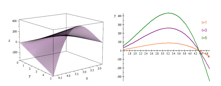
The flow of a curve is said to be inextensible if the arc length in the first case and the intrinsic curvature in the second case are preserved. In this work, we investigated the inextensible flow of a curve on $ S^2 $ according to a modified orthogonal Saban frame. Initially, we gave the definition of the modified Saban frame and then established the relations between the Frenet and the modified orthogonal Saban frames. Later, we determined the inextensible curve flow and geodesic curvature of a curve on the unit sphere using the modified orthogonal Saban frame. Also, we gave some theorems and results for special cases of the evolution of a curve on a sphere. Finally, we gave examples and their graphs for the inextensible flow equation of curvatures.
- evolution,
- inextensible flow,
- modified Saban frame,
- Saban frame,
- geodesic curvature
Citation: Atakan Tuğkan Yakut, Alperen Kızılay. On the curve evolution with a new modified orthogonal Saban frame[J]. AIMS Mathematics, 2024, 9(10): 29573-29586. doi: 10.3934/math.20241432

Related Papers:

Abstract

The flow of a curve is said to be inextensible if the arc length in the first case and the intrinsic curvature in the second case are preserved. In this work, we investigated the inextensible flow of a curve on $ S^2 $ according to a modified orthogonal Saban frame. Initially, we gave the definition of the modified Saban frame and then established the relations between the Frenet and the modified orthogonal Saban frames. Later, we determined the inextensible curve flow and geodesic curvature of a curve on the unit sphere using the modified orthogonal Saban frame. Also, we gave some theorems and results for special cases of the evolution of a curve on a sphere. Finally, we gave examples and their graphs for the inextensible flow equation of curvatures.

References

[1]	V. Parque, T. Miyashita, Smooth curve fitting of mobile robot trajectories using differential evolution, IEEE Access, 8 (2020), 82855–82866. https://doi.org/10.1109/ACCESS.2020.2991003 doi: 10.1109/ACCESS.2020.2991003
[2]	P. P. Kumar, S. Balakrishnan, A. Magesh, P. Tamizharasi, S. I. Abdelsalam, Numerical treatment of entropy generation and bejan number into an electroosmotically-driven flow of sutterby nanofluid in an asymmetric microchannel, Numer. Heat Transfer., 85 (2024), 1–20. https://doi.org/10.1080/10407790.2024.2329773 doi: 10.1080/10407790.2024.2329773
[3]	F. Lavorenti, P. Henri, F. Califano, S. Aizawa, N. Andre, Electron acceleration driven by the lower-hybrid-drift instability, Astron. Astrophys., 652 (2021), A20. https://doi.org/10.1051/0004-6361/202141049 doi: 10.1051/0004-6361/202141049
[4]	M. Desbrun, M. P. Cani, Active implicit surface for animation, Proceedings of Graphics Interface' 98, 1998. https://doi.org/10.20380/GI1998.18
[5]	F. Precioso, M. Barlaud, T. Blu, M. Unser, Smoothing $B$-spline active contour for fast and robust image and video segmentation, Proceedings 2003 International Conference on Image Processing, 2003. https://doi.org/10.1109/ICIP.2003.1246917
[6]	O. Nave, Modification of semi-analytical method applied system of ODE, Mod. Appl. Sci., 14 (2020), 75–81. https://doi.org/10.5539/mas.v14n6p75 doi: 10.5539/mas.v14n6p75
[7]	H. Q. Lu, J. S. Todhunter, T. W. Sze, Congruence conditions for nonplanar developable surfaces and their application to surface recognition, CVGIP, 58 (1993), 265–285. https://doi.org/10.1006/ciun.1993.1042 doi: 10.1006/ciun.1993.1042
[8]	G. S. Chirikjian, J. W. Burdick, A modal approach to hyper-redundant manipulator kinematics, IEEE Trans. Rob. Autom., 10 (1994), 343–354. https://doi.org/10.1109/70.294209 doi: 10.1109/70.294209
[9]	Ö. G. Yıldız, M. Tosun, S. Ö. Karakuş, A note on inextensible flows of curves in $E^n$, Int. Electron. J. Geom., 6 (2013), 118–124.
[10]	A. Kızılay, Ö. G. Yıldız, O. Z. Okuyucu, Evolution of quaternionic curve in the semi-Euclidean space $E^{4}_{2}$, Math. Methods Appl. Sci., 44 (2021), 7577–7587. https://doi.org/10.1002/mma.6374 doi: 10.1002/mma.6374
[11]	D. Y. Kwon, F. C. Park, Evolution of inelastic plane curves, Appl. Math. Lett., 12 (1999), 115–119. https://doi.org/10.1016/S0893-9659(99)00088-9 doi: 10.1016/S0893-9659(99)00088-9
[12]	D. Y. Kwon, F. C. Park, D. P. Chi, Inextensible flows of curves and developable surfaces, Appl. Math. Lett., 18 (2005), 1156–1162. https://doi.org/10.1016/j.aml.2005.02.004 doi: 10.1016/j.aml.2005.02.004
[13]	D. Latifi, A. Razavi, Inextensible flows of curves in Minkowskian space, Adv. Stud. Theor. Phys., 2 (2008), 761–768.
[14]	N. Gurbuz, Inextensible flows of spacelike, timelike and null curves, Int. J. Contemp. Mtath. Sci., 4 (2009), 1599–1604.
[15]	Ö. G. Yıldız, S. Ersoy, M. Masal, A note on inextensible flows of curves on oriented surface, Cubo (Temuco), 16 (2014), 11–19. http://doi.org/10.4067/S0719-06462014000300002 doi: 10.4067/S0719-06462014000300002
[16]	T. Sasai, The fundamental theorem of analytic space curves and apparent singularities of Fuchsian differential equations, Tohoku Math. J., 36 (1984), 17–24. https://doi.org/10.2748/tmj/1178228899 doi: 10.2748/tmj/1178228899
[17]	G. Ş. Atalay, A new approach to special curved surface families according to modified orthogonal frame, AIMS Math., 9 (2024), 20662–20676. https://doi.org/10.3934/math.20241004 doi: 10.3934/math.20241004
[18]	B. Bükcü, M. K. Karacan, On the modified orthogonal frame with curvature and torsion in 3-space, Math. Sci. Appl. E-Notes, 4 (2016), 184–188. https://doi.org/10.36753/mathenot.421429 doi: 10.36753/mathenot.421429
[19]	K. Eren, A study of the evolution of space curves with modified orthogonal frame in Euclidean 3-space, Appl. Math. E-Notes, 22 (2022), 281–286.
[20]	K. Eren, S. Ersoy, On characterization of Smarandache curves constructed by modified orthogonal frame, Math. Sci. Appl. E-Notes, 12 (2024), 101–112. https://doi.org/10.36753/mathenot.1409228 doi: 10.36753/mathenot.1409228
[21]	A. Kızılay, A. T. Yakut, A work on inextensible flows of space curves with respect to a new orthogonal frame in $E ^3$, Honam Math. J., 45 (2023), 668–677. https://doi.org/10.5831/HMJ.2023.45.4.668 doi: 10.5831/HMJ.2023.45.4.668
[22]	A. Kızılay, A. T. Yakut, Inextensible flows of space curves according to a new orthogonal frame with curvature in $E^{3}_{1}$, Int. Electron. J. Geom., 16 (2023), 577–593. https://doi.org/10.36890/iejg.1274663 doi: 10.36890/iejg.1274663
[23]	J. J. Koenderink, Solid shape, MIT Press, 1990.
[24]	K. Taşköprü, Smarandache curves on $S ^2$, Bol. Soc. Paran. Mat., 32 (2014), 51–59. https://doi.org/10.5269/bspm.v32i1.19242 doi: 10.5269/bspm.v32i1.19242
[25]	A. T. Ali, Special Smarandache curves in the Euclidean space, Int. J. Math. Combin., 2 (2010), 30–36. https://doi.org/10.5281/zenodo.9392 doi: 10.5281/zenodo.9392
[26]	A. T. Yakut, M. Savas, T. Tamirci, The Smarandache curves on $S^{2}_{1}$ and its duality on $H^{2}_{0}$, J. Appl. Math., 12 (2014), 1–12. https://doi.org/10.1155/2014/193586 doi: 10.1155/2014/193586
[27]	M. Savas, A. T. Yakut, T. Tamirci, The Smarandache curves on $H^{2}_{0}$, Gazi Univ. J. Sci., 29 (2016), 69–77.

Reader Comments

Your name:*

Email:*
© 2024 the Author(s), licensee AIMS Press. This is an open access article distributed under the terms of the Creative Commons Attribution License (http://creativecommons.org/licenses/by/4.0)