Laplacian integral signed graphs with few cycles

Dijian Wang; Dongdong Gao; Dijian Wang; Dongdong Gao

doi:10.3934/math.2023354

AIMS Mathematics

2023, Volume 8, Issue 3: 7021-7031. doi: 10.3934/math.2023354

Previous Article Next Article

Research article

Laplacian integral signed graphs with few cycles

Dijian Wang ¹,
Dongdong Gao ^{2
,
,}

1.
School of Science, Zhejiang University of Science and Technology, Hangzhou, Zhejiang, 310023, China
2.
Department of Mathematics and Computer Science, Tongling University, Tongling, Anhui 244000, China

Received: 25 October 2022 Revised: 27 December 2022 Accepted: 03 January 2023 Published: 11 January 2023
MSC : 05C50, 05C22

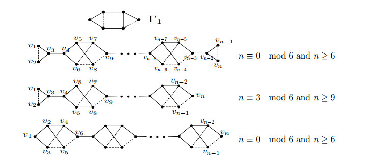
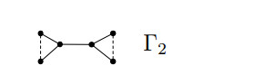
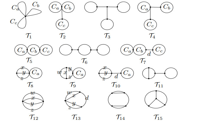
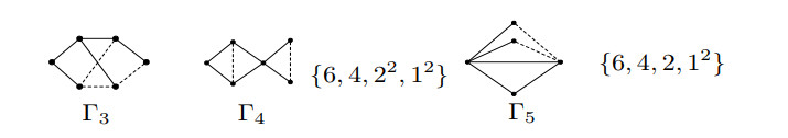
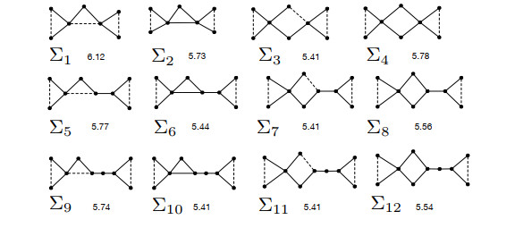
A connected graph with $ n $ vertices and $ m $ edges is called $ k $-cyclic graph if $ k = m-n+1. $ We call a signed graph is Laplacian integral if all eigenvalues of its Laplacian matrix are integers. In this paper, we will study the Laplacian integral $ k $-cyclic signed graphs with $ k = 0, 1, 2, $ $ 3 $ and determine all connected Laplacian integral signed trees, unicyclic, bicyclic and tricyclic signed graphs.
- signed graph,
- Laplacian integral graph,
- spectrum
Citation: Dijian Wang, Dongdong Gao. Laplacian integral signed graphs with few cycles[J]. AIMS Mathematics, 2023, 8(3): 7021-7031. doi: 10.3934/math.2023354

Related Papers:

Abstract

A connected graph with $ n $ vertices and $ m $ edges is called $ k $-cyclic graph if $ k = m-n+1. $ We call a signed graph is Laplacian integral if all eigenvalues of its Laplacian matrix are integers. In this paper, we will study the Laplacian integral $ k $-cyclic signed graphs with $ k = 0, 1, 2, $ $ 3 $ and determine all connected Laplacian integral signed trees, unicyclic, bicyclic and tricyclic signed graphs.

References

[1]	M. Andeli$\acute{c}, $ T. Koledin, Z. Stani$\acute{c}, $ On regular signed graphs with three eigenvalues, Discuss. Math. Graph Theory, 40 (2020), 405–416. http://dx.doi.org/10.7151/dmgt.2279 doi: 10.7151/dmgt.2279
[2]	F. Belardo, S. Cioab$\breve{a}$, J. Koolen, J. F. Wang, Open problems in the spectral theory of signed graphs, Art Discrete Appl. Math., 1 (2018), #P2.10. http://dx.doi.org/10.26493/2590-9770.1286.d7b
[3]	F. Belardo, P. Petecki, J. Wang, On signed graphs whose second largest Laplacian eigenvalue does not exceed 3, Linear Multilinear A., 64 (2016), 1–15. http://dx.doi.org/10.1080/03081087.2015.1120701 doi: 10.1080/03081087.2015.1120701
[4]	D. Cvetković, I. Gutman, N. Trinajstić, Conjugated molecules having integral graph spectra, Chem. Phys. Letters, 29 (1974), 65–68. http://dx.doi.org/10.1016/0009-2614(74)80135-1 doi: 10.1016/0009-2614(74)80135-1
[5]	D. Cvetković, S. Simić, D. Stevanović, 4-regular integral graphs, Univ. Beograd, Publ. Elektrotehn. Fak. Ser. Mat., 9 (1998), 89–102. Available from: https://www.researchgate.net/publication/228847421_4-regular_integral_graphs/citations.
[6]	S. Fallat, H. Lerch, J. Molitierno, M. Neumann, On the graphs whose Laplacian matrices have distinct integer eigenvalue, J. Graph theory., 50 (2005), 162–174. http://dx.doi.org/10.1002/jgt.20102 doi: 10.1002/jgt.20102
[7]	K. A. Germina, S. K. Hameed, T. Zaslavsky, On products and line graphs of signed graphs, their eigenvalues and energy, Linear Algebra Appl., 435 (2010), 2432–2450. http://dx.doi.org/10.1016/j.laa.2010.10.026 doi: 10.1016/j.laa.2010.10.026
[8]	F. Harary, A. J. Schwenk, Which graphs have integral spectra?, Graphs and Combinatorics, (R. Bari, F. Harary, Eds.) Springer-Verlag, Berlin, (1974), 45–51. http://dx.doi.org/10.1007/BFb0066434
[9]	R. Merris, Degree maximal graphs are Laplacian integral, Linear Algebra Appl., 199 (1994), 381–389. http://dx.doi.org/10.1016/0024-3795(94)90361-1 doi: 10.1016/0024-3795(94)90361-1
[10]	S. G. Guo, Y. F. Wang, The Laplacian spectral radius of tricyclic graphs with $n$ vertices and $k$ pendent vertices, Linear Algebra Appl., 431 (2009), 139–147. http://dx.doi.org/10.1016/j.laa.2007.12.013 doi: 10.1016/j.laa.2007.12.013
[11]	Y. Hou, J. Li, Y. Pan, On the Laplacian eigenvalues of signed graphs, Linear Multilinear A., 51 (2003), 21–30. http://dx.doi.org/10.1080/0308108031000053611 doi: 10.1080/0308108031000053611
[12]	X. Huang, Q. Huang, F. Wen, On the Laplacian integral tricyclic graphs, Linear Multilinear Algebra., 63 (2015), 1356–1371. http://dx.doi.org/10.1080/03081087.2014.936436 doi: 10.1080/03081087.2014.936436
[13]	J. Zhang, Q. Huang, C. Song, X. Huang, $Q$-integral unicyclic, bicyclic and tricyclic graphs, Math. Nachr., (2016), 1–10. http://dx.doi.org/10.1002/mana.201500313
[14]	S. Kirkland, Laplacian integral graphs with maximum degree 3, Electron. J. Combin., 15 (2008), R120. http://dx.doi.org/10.1002/nme.2324 doi: 10.1002/nme.2324
[15]	M. Liu, B. Liu, Some results on the Laplacian spectrum, Comput. Math. Appl., 59 (2010), 3612–3616. http://dx.doi.org/10.1016/j.camwa.2010.03.058 doi: 10.1016/j.camwa.2010.03.058
[16]	A. J. Schwenk, Exactly thirteen connected cubic graphs have integral spectra, In: Theor. Appl. Graphs, Proc., Kalamazoo, 1976, Lecture Notes in Math., 642 (1978), 516–533. http://dx.doi.org/10.1007/BFb0070407
[17]	Z. Stani$\acute{c}, $ Integral regular net-balanced signed graphs with vertex degree at most four, Ars Math. Contemp., 17 (2019), 103–114. http://dx.doi.org/10.26493/1855-3974.1740.803 doi: 10.26493/1855-3974.1740.803
[18]	D. Wang, Y. Hou, Integral signed subcubic graphs, Linear Algebra Appl., 593 (2020), 29–44. http://dx.doi.org/10.1016/j.laa.2020.01.037 doi: 10.1016/j.laa.2020.01.037
[19]	D. Wang, Y. Hou, Laplacian integral signed subcubic graphs, Electron. J. Linear Al., 37 (2021), 163–176. http://dx.doi.org/10.13001/ELA.2021.5699. doi: 10.13001/ELA.2021.5699
[20]	T. Zaslavsky, Signed graphs, Discrete Appl. Math. 4 (1982) 47–74. http://dx.doi.org/10.1016/0166-218x(82)90033-6

Reader Comments

Your name:*

Email:*
© 2023 the Author(s), licensee AIMS Press. This is an open access article distributed under the terms of the Creative Commons Attribution License (http://creativecommons.org/licenses/by/4.0)