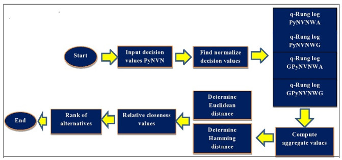
The article explores multiple attribute decision making problems through the use of the Pythagorean neutrosophic vague normal set (PyNVNS). The PyNVNS can be generalized to the Pythagorean neutrosophic interval valued normal set (PyNIVNS) and vague set. This study discusses $ q $-rung log Pythagorean neutrosophic vague normal weighted averaging ($ q $-rung log PyNVNWA), $ q $-rung logarithmic Pythagorean neutrosophic vague normal weighted geometric ($ q $-rung log PyNVNWG), $ q $-rung log generalized Pythagorean neutrosophic vague normal weighted averaging ($ q $-rung log GPyNVNWA), and $ q $-rung log generalized Pythagorean neutrosophic vague normal weighted geometric ($ q $-rung log GPyNVNWG) sets. The properties of $ q $-rung log PyNVNSs are discussed based on algebraic operations. The field of agricultural robotics can be described as a fusion of computer science and machine tool technology. In addition to crop harvesting, other agricultural uses are weeding, aerial photography with seed planting, autonomous robot tractors and soil sterilization robots. This study entailed selecting five types of agricultural robotics at random. There are four types of criteria to consider when choosing a robotics system: robot controller features, cheap off-line programming software, safety codes and manufacturer experience and reputation. By comparing expert judgments with the criteria, this study narrows the options down to the most suitable one. Consequently, $ q $ has a significant effect on the results of the models.
Citation: Murugan Palanikumar, Chiranjibe Jana, Biswajit Sarkar, Madhumangal Pal. $ q $-rung logarithmic Pythagorean neutrosophic vague normal aggregating operators and their applications in agricultural robotics[J]. AIMS Mathematics, 2023, 8(12): 30209-30243. doi: 10.3934/math.20231544
The article explores multiple attribute decision making problems through the use of the Pythagorean neutrosophic vague normal set (PyNVNS). The PyNVNS can be generalized to the Pythagorean neutrosophic interval valued normal set (PyNIVNS) and vague set. This study discusses $ q $-rung log Pythagorean neutrosophic vague normal weighted averaging ($ q $-rung log PyNVNWA), $ q $-rung logarithmic Pythagorean neutrosophic vague normal weighted geometric ($ q $-rung log PyNVNWG), $ q $-rung log generalized Pythagorean neutrosophic vague normal weighted averaging ($ q $-rung log GPyNVNWA), and $ q $-rung log generalized Pythagorean neutrosophic vague normal weighted geometric ($ q $-rung log GPyNVNWG) sets. The properties of $ q $-rung log PyNVNSs are discussed based on algebraic operations. The field of agricultural robotics can be described as a fusion of computer science and machine tool technology. In addition to crop harvesting, other agricultural uses are weeding, aerial photography with seed planting, autonomous robot tractors and soil sterilization robots. This study entailed selecting five types of agricultural robotics at random. There are four types of criteria to consider when choosing a robotics system: robot controller features, cheap off-line programming software, safety codes and manufacturer experience and reputation. By comparing expert judgments with the criteria, this study narrows the options down to the most suitable one. Consequently, $ q $ has a significant effect on the results of the models.

| [1] |
A. Kaplan, M. Haenlein, Rulers of the world, unite! The challenges and opportunities of artificial intelligence, Bus. Horizons, 63 (2020), 37–50. http://doi.org/10.1016/j.bushor.2019.09.003 doi: 10.1016/j.bushor.2019.09.003

|
| [2] |
H. Margetts, C. Dorobantu, Rethink government with AI, Nature, 568 (2019), 163–165. http://doi.org/10.1038/d41586-019-01099-5 doi: 10.1038/d41586-019-01099-5
|
| [3] |
K. Cresswell, M. Callaghan, S. Khan, Z. Sheikh, H. Mozaffar, A. Sheikh, Investigating the use of data-driven artificial intelligence in computerised decision support systems for health and social care: A systematic review, Health Inf. J., 26 (2020), 2138–2147. https://doi.org/10.1177/1460458219900452 doi: 10.1177/1460458219900452
|
| [4] | S. A. Yablonsky, Multidimensional data-driven artificial intelligence innovation, Technol. Innov. Magag. Rev., 9 (2019), 16–28. |
| [5] |
J. Klinger, J. Mateos Garcia, K. Stathoulopoulos, Deep learning, deep change? Mapping the development of the artificial intelligence general purpose technology, Scientometrics, 126 (2021), 5589–5621. http://doi.org/10.1007/s11192-021-03936-9 doi: 10.1007/s11192-021-03936-9
|
| [6] | V. Rasskazov, Financial and economic consequences of distribution of artificial intelligence as a general-purpose technology, Financ.: Theory Pract., 24 (2020), 120–132. |
| [7] |
A. Agostini, C. Torras, F. Worgotter, Efficient interactive decision-making framework for robotic applications, Artif. Intell., 247 (2017), 187–212. http://doi.org/10.1016/j.artint.2015.04.004 doi: 10.1016/j.artint.2015.04.004
|
| [8] |
L. A. Zadeh, Fuzzy sets, Inform. Control, 8 (1965), 338–353. http://doi.org/10.1016/S0019-9958(65)90241-X doi: 10.1016/S0019-9958(65)90241-X
|
| [9] |
K. Atanassov, Intuitionistic fuzzy sets, Fuzzy Sets Syst., 20 (1986), 87–96. http://doi.org/10.1016/S0165-0114(86)80034-3 doi: 10.1016/S0165-0114(86)80034-3
|
| [10] |
M. Gorzalczany, A method of inference in approximate reasoning based on interval valued fuzzy sets, Fuzzy Sets Syst., 21 (1987), 1–17. http://doi.org/10.1016/0165-0114(87)90148-5 doi: 10.1016/0165-0114(87)90148-5
|
| [11] | R. Biswas, Vague Groups, Int. J. Comput. Cogn., 4 (2006), 20–23. |
| [12] |
R. R. Yager, Pythagorean membership grades in multi criteria decision-making, IEEE T. Fuzzy Sets Syst., 22 (2014), 958–965. http://doi.org/10.1109/TFUZZ.2013.2278989 doi: 10.1109/TFUZZ.2013.2278989
|
| [13] | X. Peng, Y. Yang, Fundamental properties of interval valued Pythagorean fuzzy aggregation operators, Int. J. Int. Syst., 31 (2016), 444–487. |
| [14] |
S. Ashraf, S. Abdullah, T. Mahmood, F. Ghani, T. Mahmood, Spherical fuzzy sets and their applications in multi-attribute decision making problems, J. Intell. Fuzzy Syst., 36 (2019), 2829–2844. http://doi.org/10.3233/JIFS-172009 doi: 10.3233/JIFS-172009
|
| [15] |
A. Nicolescu, M. Teodorescu, A unifying field in logics - Book review, Int. Lett. Soc. Humanistic Sci., 43 (2015), 48–59. http://doi.org/10.18052/www.scipress.com/ILSHS.43.48 doi: 10.18052/www.scipress.com/ILSHS.43.48
|
| [16] | R. N. Xu, Regression prediction for fuzzy time series, Appl. Math. J. Chin. Univ. Ser. B, 16 (2001), 124376140. |
| [17] |
R. R. Yager, Generalized orthopair fuzzy sets, IEEE T. Fuzzy Syst., 25 (2016), 1222–1230. http://doi.org/10.1109/TFUZZ.2016.2604005 doi: 10.1109/TFUZZ.2016.2604005
|
| [18] |
B. P. Joshi, A. Singh, P. K. Bhatt, K. S. Vaisla, Interval valued $q$-rung orthopair fuzzy sets and their properties, J. Intell. Fuzzy Syst., 35 (2018), 5225–5230. http://doi.org/10.3233/JIFS-169806 doi: 10.3233/JIFS-169806
|
| [19] |
R. R. Yager, Generalized orthopair fuzzy sets, IEEE T. Fuzzy Syst., 25 (2017), 1222–1230. http://doi.org/10.1109/TFUZZ.2016.2604005 doi: 10.1109/TFUZZ.2016.2604005
|
| [20] |
M. S. Habib, O. Asghar, A. Hussain, M. Imran, M. P. Mughal, B. Sarkar, A robust possibilistic programming approach toward animal fat-based biodiesel supply chain network design under uncertain environment, J. Clean. Prod., 278 (2021), 122403. http://doi.org/10.1016/j.jclepro.2020.122403 doi: 10.1016/j.jclepro.2020.122403
|
| [21] |
B. Sarkar, M. Tayyab, N. Kim, M. S. Habib, Optimal production delivery policies for supplier and manufacturer in a constrained closed-loop supply chain for returnable transport packaging through metaheuristic approach, Comput. Ind. Eng., 135 (2019), 987–1003. http://doi.org/10.1016/j.cie.2019.05.035 doi: 10.1016/j.cie.2019.05.035
|
| [22] |
D. Yadav, R. Kumari, N. Kumar, B. Sarkar, Reduction of waste and carbon emission through the selection of items with crossprice elasticity of demand to form a sustainable supply chain with preservation technology, J. Clean. Prod., 297 (2019), 126298. http://doi.org/10.1016/j.jclepro.2021.126298 doi: 10.1016/j.jclepro.2021.126298
|
| [23] |
B. K. Dey, S. Bhuniya, B. Sarkar, Involvement of controllable lead time and variable demand for a smart manufacturing system under a supply chain management, Expert Syst. Appl., 184 (2021), 115464. http://doi.org/10.1016/j.eswa.2021.115464 doi: 10.1016/j.eswa.2021.115464
|
| [24] | B. C. Cuong, V. Kreinovich, Picture fuzzy sets-A new concept for computational intelligence problems, 2013 Third World Congress on Information and Communication Technologies, 2013. http://doi.org/10.1109/WICT.2013.7113099 |
| [25] |
M. Akram, W. A. Dudek, F. Ilyas, Group decision making based on Pythagorean fuzzy TOPSIS method, Int. J. Intell. Syst., 34 (2019), 1455–1475. http://doi.org/10.1002/int.22103 doi: 10.1002/int.22103
|
| [26] |
M. Akram, W. A. Dudek, J. M. Dar, Pythagorean Dombi Fuzzy Aggregation Operators with Application in Multi-criteria Decision-making, Int. J. Intell. Syst., 34 (2019), 3000–3019. http://doi.org/10.1002/int.22183 doi: 10.1002/int.22183
|
| [27] | Z. Xu, Intuitionistic fuzzy aggregation operators, IEEE Transactions on Fuzzy Systems, (2007), 1179–1187. |
| [28] |
W. F. Liu, J. Chang, X. He, Generalized Pythagorean fuzzy aggregation operators and applications in decision making, Control Decision, 31 (2016), 2280–2286. http://doi.org/10.13195/j.kzyjc.2015.1537 doi: 10.13195/j.kzyjc.2015.1537
|
| [29] |
K. Rahman, S. Abdullah, M. Shakeel, M. S. A. Khan, M. Ullah, Interval valued Pythagorean fuzzy geometric aggregation operators and their application to group decision-making problem, Cogent Math., 4 (2017), 1338638. http://doi.org/10.1080/23311835.2017.1338638 doi: 10.1080/23311835.2017.1338638
|
| [30] |
K. Rahman, A. Ali, S. Abdullah, F. Amin, Approaches to multi-attribute group decision-making based on induced interval valued Pythagorean fuzzy Einstein aggregation operator, New Math. Natural Comput., 14 (2018), 343–361. https://doi.org/10.1142/S1793005718500217 doi: 10.1142/S1793005718500217
|
| [31] |
Z. Yang, J. Chang, Interval-valued Pythagorean normal fuzzy information aggregation operators for multiple attribute decision making approach, IEEE Access, 8 (2020), 51295–51314. http://doi.org/10.1109/ACCESS.2020.2978976 doi: 10.1109/ACCESS.2020.2978976
|
| [32] |
K. G. Fatmaa, K. Cengiza, Spherical fuzzy sets and spherical fuzzy TOPSIS method, J. Intell. Fuzzy Syst., 36 (2019), 337–352. http://doi.org/10.3233/JIFS-181401 doi: 10.3233/JIFS-181401
|
| [33] |
P. Liu, G. Shahzadi, M. Akram, Specific types of q-rung picture fuzzy Yager aggregation operators for decision-making, Int. J. Comput. Intell. Syst., 13 (2020), 1072–1091. http://doi.org/10.2991/ijcis.d.200717.001 doi: 10.2991/ijcis.d.200717.001
|
| [34] |
Z. Yang, X. Li, Z. Cao, J. Li, $q$-rung orthopair normal fuzzy aggregation operators and their application in multi attribute decision-making, Mathematics, 7 (2019), 1142. http://doi.org/10.3390/math7121142 doi: 10.3390/math7121142
|
| [35] |
R. R. Yager, N. Alajlan, Approximate reasoning with generalized orthopair fuzzy sets, Inform. Fusion., 38 (2017), 65–73. http://doi.org/10.1016/j.inffus.2017.02.005 doi: 10.1016/j.inffus.2017.02.005
|
| [36] |
M. I. Ali, Another view on q-rung orthopair fuzzy sets, Int. J. Intell. Syst., 33 (2019), 2139–2153. http://doi.org/10.1002/int.22007 doi: 10.1002/int.22007
|
| [37] |
P. Liu, P. Wang, Some $q$-rung orthopair fuzzy aggregation operators and their applications to multiple-attribute decision making, Int. J. Intell. Syst., 33 (2018), 259–280. http://doi.org/10.1002/int.21927 doi: 10.1002/int.21927
|
| [38] |
P. Liu, J. Liu, Some $q$-rung orthopai fuzzy Bonferroni mean operators and their application to multi-attribute group decision making, Int. J. Intell. Syst., 33 (2018), 315–347. http://doi.org/10.1002/int.21933 doi: 10.1002/int.21933
|
| [39] |
C. Jana, G. Muhiuddin, M. Pal, Some Dombi aggregation of $q$-rung orthopair fuzzy numbers in multiple-attribute decision making, Int. J. Intell. Syst., 34 (2019), 3220–3240. http://doi.org/10.1002/int.22191 doi: 10.1002/int.22191
|
| [40] |
J. Wang, R. Zhang, X. Zhu, Z. Zhou, X. Shang, W. Li, Some $q$-rung orthopair fuzzy Muirhead means with their application to multi-attribute group decision making, J. Intell. Fuzzy Syst., 36 (2019), 1599–1614. http://doi.org/10.3233/JIFS-18607 doi: 10.3233/JIFS-18607
|
| [41] |
M. S. Yang, C. H. Ko, On a class of fuzzy c-numbers clustering procedures for fuzzy data, Fuzzy Sets. Syst., 84 (1996), 49–60. http://doi.org/10.1016/0165-0114(95)00308-8 doi: 10.1016/0165-0114(95)00308-8
|
| [42] |
A. Hussain, M. I. Ali, T. Mahmood, Hesitant $q$-rung orthopair fuzzy aggregation operators with their applications in multi-criteria decision making, Iran. J. Fuzzy Syst., 17 (2020), 117–134. http://doi.org/10.22111/IJFS.2020.5353 doi: 10.22111/IJFS.2020.5353
|
| [43] |
A. Hussain, M. I. Ali, T. Mahmood, M. Munir, Group based generalized $q$-rung orthopair average aggregation operators and their applications in multi-criteria decision making, Complex Intell. Syst., 7 (2021), 123–144. http://doi.org/10.1007/s40747-020-00176-x doi: 10.1007/s40747-020-00176-x
|
| [44] | F. Smarandache, A unifying field in logics, Neutrosophy neutrosophic probability, set and logic, 2 Eds., Rehoboth: American Research Press, 1999. |
| [45] |
J. Ye, Similarity measures between interval neutrosophic sets and their applications in Multi-criteria decision-making, J. Intell. Fuzzy Syst., 26 (2014), 165–172. http://doi.org/10.3233/IFS-120724 doi: 10.3233/IFS-120724
|
| [46] |
H. Zhang, J. Wang, X. Chen, Interval neutrosophic sets and its application in multi-criteria decision making problems, Sci. World J., 2014 (2014), 645953. http://doi.org/10.1155/2014/645953 doi: 10.1155/2014/645953
|
| [47] |
H. Bustince, P. Burillo, Vague sets are intuitionistic fuzzy sets, Fuzzy Sets Syst., 79 (1996), 403–405. http://doi.org/10.1016/0165-0114(95)00154-9 doi: 10.1016/0165-0114(95)00154-9
|
| [48] |
A. Kumar, S. P. Yadav, S. Kumar, Fuzzy system reliability analysis using $T$ based arithmetic operations on $LR$ type interval valued vague sets, Int. J. Qual. Reliab. Manag., 24 (2007), 846–860. http://doi.org/10.1108/02656710710817126 doi: 10.1108/02656710710817126
|
| [49] |
J. Wang, S. Y. Liu, J. Zhang, S. Y. Wang, On the parameterized OWA operators for fuzzy MCDM based on vague set theory, Fuzzy Optim. Decis. Making, 5 (2006), 5–20. http://doi.org/10.1007/s10700-005-4912-2 doi: 10.1007/s10700-005-4912-2
|
| [50] |
X. Zhang, Z. Xu, Extension of TOPSIS to multiple criteria decision-making with Pythagorean fuzzy sets, Int. J. Intell. Syst., 29 (2014), 1061–1078. http://doi.org/10.1002/int.21676 doi: 10.1002/int.21676
|
| [51] | C. L. Hwang, K. Yoon, Multiple Attribute Decision Making-Methods and Applications, A State-of-the-Art Survey, Berlin, Heidelberg: Springer, 1981. http://doi.org/10.1007/978-3-642-48318-9 |
| [52] |
C. Jana, M. Pal, Application of bipolar intuitionistic fuzzy soft sets in decision-making problem, Int. J. Fuzzy Syst. Appl., 7 (2018), 32–55. http://doi.org/10.4018/IJFSA.2018070103 doi: 10.4018/IJFSA.2018070103
|
| [53] |
C. Jana, Multiple attribute group decision-making method based on extended bipolar fuzzy MABAC approach, Comput. Appl. Math., 40 (2021), 227. http://doi.org/10.1007/s40314-021-01606-3 doi: 10.1007/s40314-021-01606-3
|
| [54] |
C. Jana, M. Pal, A Robust single valued neutrosophic soft aggregation operators in multi criteria decision-making, Symmetry, 11 (2019), 110. http://doi.org/10.3390/sym11010110 doi: 10.3390/sym11010110
|
| [55] |
C. Jana, T. Senapati, M. Pal, Pythagorean fuzzy Dombi aggregation operators and its applications in multiple attribute decision-making, Int. J. Intell. Syst., 34 (2019), 2019–2038. http://doi.org/10.1002/int.22125 doi: 10.1002/int.22125
|
| [56] |
K. Ullah, T. Mahmood, Z. Ali, N. Jan, On some distance measures of complex Pythagorean fuzzy sets and their applications in pattern recognition, Comput. Intell. Syst., 6 (2020), 15–27. http://doi.org/10.1007/s40747-019-0103-6 doi: 10.1007/s40747-019-0103-6
|
| [57] |
C. Jana, M. Pal, F. Karaaslan, J. Q. Wang, Trapezoidal neutrosophic aggregation operators and their application to the multi-attribute decision-making process, Sci. Iran., 27 (2020), 1655–1673. http://doi.org/10.24200/SCI.2018.51136.2024 doi: 10.24200/SCI.2018.51136.2024
|
| [58] |
C. Jana, M. Pal, Multi criteria decision-making process based on some single valued neutrosophic dombi power aggregation operators, Soft Comput., 25 (2021), 5055–5072. http://doi.org/10.1007/s00500-020-05509-z doi: 10.1007/s00500-020-05509-z
|
| [59] |
M. Palanikumar, K. Arulmozhi, C. Jana, M. Pal, Multiple‐attribute decision-making spherical vague normal operators and their applications for the selection of farmers, Expert Syst., 40 (2023), e13188. http://doi.org/10.1111/exsy.13188 doi: 10.1111/exsy.13188
|
| [60] |
V. Uluçay, Q-neutrosophic soft graphs in operations management and communication network, Soft Comput., 25 (2021), 8441–8459. http://doi.org/10.1007/s00500-021-05772-8 doi: 10.1007/s00500-021-05772-8
|
| [61] |
V. Uluçay, Some concepts on interval-valued refined neutrosophic sets and their applications, J. Ambient Intell. Human. Comput., 12 (2021), 7857–7872. http://doi.org/10.1007/s12652-020-02512-y doi: 10.1007/s12652-020-02512-y
|
| [62] |
V. Uluçay, I. Deli, M. Şahin, Similarity measures of bipolar neutrosophic sets and their application to multiple criteria decision making, Neural Comput. Appl., 29 (2021), 739–748. http://doi.org/10.1007/s00521-016-2479-1 doi: 10.1007/s00521-016-2479-1
|
| [63] |
M. Sahin, N. Olgun, V. Uluçay, H. Acioglu, Some weighted arithmetic operators and geometric operators with SVNSs and their application to multi-criteria decision making problems, New Trends Neutrosophic Theory Appl., 2 (2018), 85–104. http://doi.org/10.5281/zenodo.1237953 doi: 10.5281/zenodo.1237953
|
| [64] | M. Sahin, N. Olgun, V. Uluçay, A. Kargin, F. Smarandache, A new similarity measure based on falsity value between single valued neutrosophic sets based on the centroid points of transformed single valued neutrosophic numbers with applications to pattern recognition, Neutrosophic Sets Syst., 15 (2017), 31–48. |
| [65] |
Y. Lu, Y. Xu, E. H. Viedma, Consensus progress for large-scale group decision making in social networks with incomplete probabilistic hesitant fuzzy information, Appl. Soft Comput., 126 (2022), 109249. http://doi.org/10.1016/j.asoc.2022.109249 doi: 10.1016/j.asoc.2022.109249
|
| [66] |
Y. Lu, Y. Xu, J. Huang, J. Wei, E. H. Viedma, Social network clustering and consensus-based distrust behaviors management for large scale group decision-making with incomplete hesitant fuzzy preference relations, Appl. Soft Comput., 117 (2022), 108373. http://doi.org/10.1016/j.asoc.2021.108373 doi: 10.1016/j.asoc.2021.108373
|
| [67] |
C. Jana, G. Muhiuddin, M. Pal, Multi-criteria decision-making approach based on SVTrN Dombi aggregation functions. Artif. Intell. Rev., 54 (2021), 3685–3723. http://doi.org/10.1007/s10462-020-09936-0 doi: 10.1007/s10462-020-09936-0
|
| [68] |
M. Palanikumar, K. Arulmozhi, C. Jana, Multiple attribute decision-making approach for Pythagorean neutrosophic normal interval-valued aggregation operators, Comput. Appl. Math., 41 (2022), 90. http://doi.org/10.1007/s40314-022-01791-9 doi: 10.1007/s40314-022-01791-9
|
| [69] |
X. Peng, H. Yuan, Fundamental properties of Pythagorean fuzzy aggregation operators, Int. J. Intell. Syst. 31 (2016), 444–487. http://doi.org/10.1002/int.21790 doi: 10.1002/int.21790
|
| [70] |
B. Sarkar, M. Omair, N. Kim, A cooperative advertising collaboration policy in supply chain management under uncertain conditions, Appl. Soft Comput., 88 (2020), 105948. http://doi.org/10.1016/j.asoc.2019.105948 doi: 10.1016/j.asoc.2019.105948
|
| [71] |
U. Mishra, J. Z. Wu, B. Sarkar, Optimum sustainable inventory management with backorder and deterioration under controllable carbon emissions, J. Clean. Prod., 279 (2021), 123699. http://doi.org/10.1016/j.jclepro.2020.123699 doi: 10.1016/j.jclepro.2020.123699
|
| [72] |
B. Sarkar, M. Sarkar, B. Ganguly, L. E. Cárdenas-Barrón, Combined effects of carbon emission and production quality improvement for fixed lifetime products in a sustainable supply chain management, Int. J. Prod. Econ., 231 (2021), 107867. http://doi.org/10.1016/j.ijpe.2020.107867 doi: 10.1016/j.ijpe.2020.107867
|
| [73] |
U. Mishra, J. Z. Wu, B. Sarkar, A sustainable production-inventory model for a controllable carbon emissions rate under shortages, J. Clean. Prod., 256 (2020), 120268. http://doi.org/10.1016/j.jclepro.2020.120268 doi: 10.1016/j.jclepro.2020.120268
|
| [74] |
M. Ullah, B. Sarkar, Recovery-channel selection in a hybrid manufacturing-remanufacturing production model with RFID and product quality, Int. J. Prod. Econ., 219 (2020), 360–374. http://doi.org/10.1016/j.ijpe.2019.07.017 doi: 10.1016/j.ijpe.2019.07.017
|
| [75] |
M. Ullah, I. Asghar, M. Zahid, M. Omair, A. AlArjani, B. Sarkar, Ramification of remanufacturing in a sustainable three-echelon closed-loop supply chain management for returnable products, J. Clean. Prod., 290 (2021), 125609. http://doi.org/10.1016/j.jclepro.2020.125609 doi: 10.1016/j.jclepro.2020.125609
|


Figures(4) / Tables(1)

Murugan Palanikumar, Chiranjibe Jana, Biswajit Sarkar, Madhumangal Pal. $ q $-rung logarithmic Pythagorean neutrosophic vague normal aggregating operators and their applications in agricultural robotics[J]. AIMS Mathematics, 2023, 8(12): 30209-30243. doi: 10.3934/math.20231544


 DownLoad: