Modeling the implications of nitric oxide dynamics on information transmission: An automata networks approach

Pablo Fernández-López; Patricio García Báez; Ylermi Cabrera-León; Aleš Procházka; Carmen Paz Suárez-Araujo; Pablo Fernández-López; Patricio García Báez; Ylermi Cabrera-León; Aleš Procházka; Carmen Paz Suárez-Araujo

doi:10.3934/math.20231541

AIMS Mathematics

2023, Volume 8, Issue 12: 30142-30181. doi: 10.3934/math.20231541

Previous Article Next Article

Research article

Modeling the implications of nitric oxide dynamics on information transmission: An automata networks approach

1.
Instituto Universitario de Cibernética, Empresa y Sociedad, Universidad de Las Palmas de Gran Canaria, Campus Universitario de Tafira, Las Palmas de Gran Canaria, 35017, Spain
2.
Departamento de Ingeniería Informática y de Sistemas, Universidad de La Laguna, Camino San Francisco de Paula, 19, San Cristóbal de La Laguna, 38200, Spain
3.
Department of Computing and Control Engineering, Univ. of Chemistry and Technology at Prague & Czech Inst. Inf., Rob. Cyber, Czech Tech Univ. of Prague, 16000 Prague, Czech Republic

Received: 15 August 2023 Revised: 17 October 2023 Accepted: 23 October 2023 Published: 06 November 2023
MSC : 92B20, 92B25, 92C20

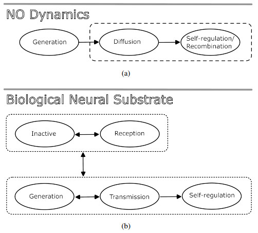
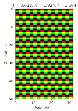
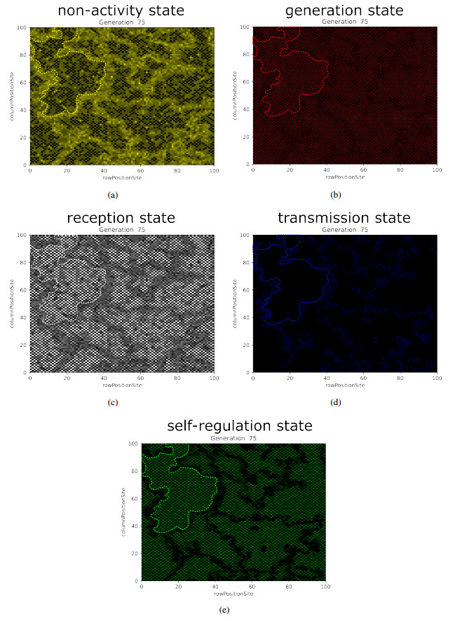
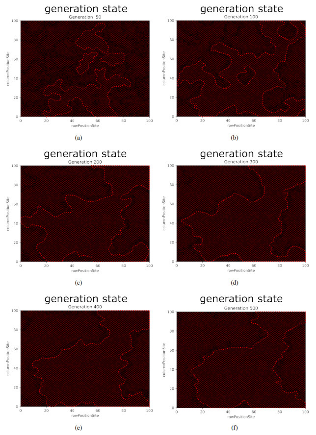
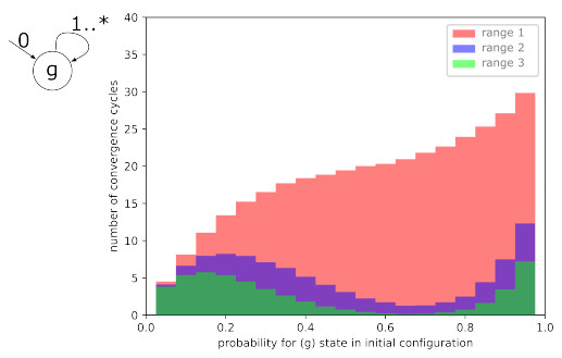
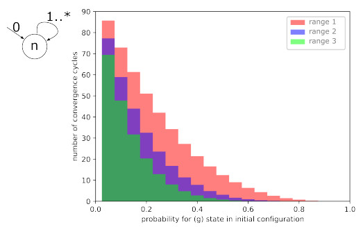
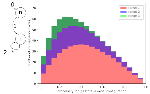
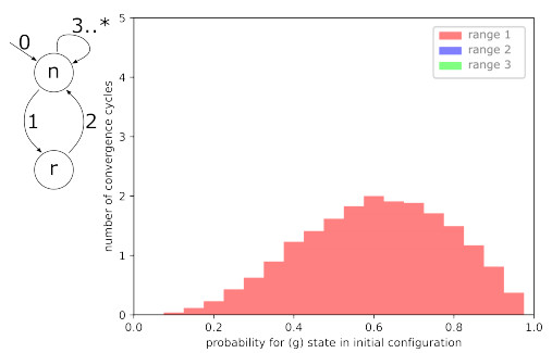
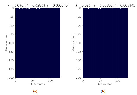
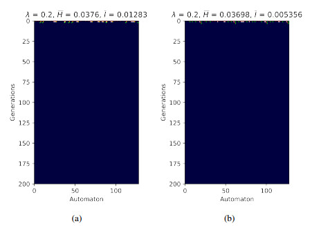
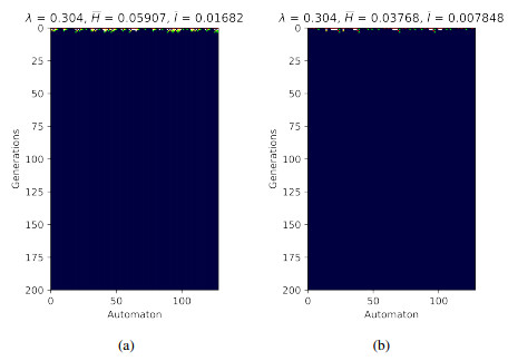
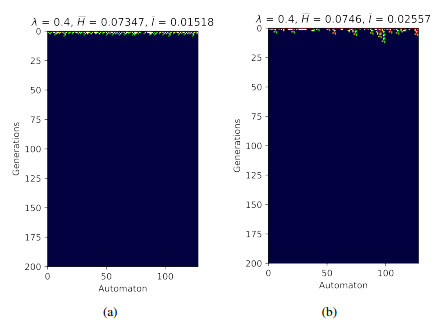
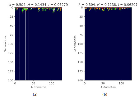
Nitric oxide (NO) is already recognized as an important signaling molecule in the brain. It diffuses easily and the nervous cell's membrane is permeable to NO. The information transmission is three-dimensional, which is different from synaptic transmission. NO operates in two different ways: Close and specific at the synapses of neurons, and as a volumetric transmitter sending signals to various targets, regardless of their anatomy, connectivity or function, when multiple nearby sources act simultaneously. These modes of operation seem to be the basis by which NO is involved in many central mechanisms of the brain, such as learning, memory formation, brain development and synaptogenesis. This work focuses on the effect of NO dynamics on the environment through which it diffuses, using automata networks. We study their implications in the formation of complex functional structures in the volume transmission (VT), which are necessary for the synchronous functional recruitment of neuronal populations. We qualitatively and quantitatively analyze the proposed model regarding these characteristics through the concepts of entropy and mutual information. The proposed deterministic model allows the incorporation of fuzzy dynamics. With that, a generalized model based on fuzzy automata networks can be provided. This allows the generation and diffusion processes of NO to be arbitrarily produced and maintained over time. This model can accommodate arbitrary processes in decision-making mechanisms and can be part of a complete formal VT framework in the brain and artificial neural networks.
- nitric oxide dynamics,
- volume transmission,
- automata network,
- mathematical modeling
Citation: Pablo Fernández-López, Patricio García Báez, Ylermi Cabrera-León, Aleš Procházka, Carmen Paz Suárez-Araujo. Modeling the implications of nitric oxide dynamics on information transmission: An automata networks approach[J]. AIMS Mathematics, 2023, 8(12): 30142-30181. doi: 10.3934/math.20231541

Related Papers:

Abstract

Nitric oxide (NO) is already recognized as an important signaling molecule in the brain. It diffuses easily and the nervous cell's membrane is permeable to NO. The information transmission is three-dimensional, which is different from synaptic transmission. NO operates in two different ways: Close and specific at the synapses of neurons, and as a volumetric transmitter sending signals to various targets, regardless of their anatomy, connectivity or function, when multiple nearby sources act simultaneously. These modes of operation seem to be the basis by which NO is involved in many central mechanisms of the brain, such as learning, memory formation, brain development and synaptogenesis. This work focuses on the effect of NO dynamics on the environment through which it diffuses, using automata networks. We study their implications in the formation of complex functional structures in the volume transmission (VT), which are necessary for the synchronous functional recruitment of neuronal populations. We qualitatively and quantitatively analyze the proposed model regarding these characteristics through the concepts of entropy and mutual information. The proposed deterministic model allows the incorporation of fuzzy dynamics. With that, a generalized model based on fuzzy automata networks can be provided. This allows the generation and diffusion processes of NO to be arbitrarily produced and maintained over time. This model can accommodate arbitrary processes in decision-making mechanisms and can be part of a complete formal VT framework in the brain and artificial neural networks.

References

[1]	R. F. Furchgott, J. V. Zawadzki, The obligatory role of endothelial cells in the relaxation of arterial smooth muscle by ACH, Nature, 288 (1980), 372–376. https://doi.org/10.1038/288373a0 doi: 10.1038/288373a0
[2]	R. F. Furchgott, J. V. Zawadzki, P. D. Cherry, Role of endothelium in the vasodilator response to acetylcholine, Vasodilatation, Edited by P. M. Vanhoutte and I. Leusen, New York: Raven Press, 1981, 49–66.
[3]	L. J. Ignarro, G. M. Buga, K. S. Wood, R. E. Byrns, G. Chaudhuri, Endothelium-derived relaxing factor produced and released from artery and vein is nitric oxide, P. Natl. Acad. Sci. USA, 84 (1987), 9265–9269. https://doi.org/10.1073/pnas.84.24.9265 doi: 10.1073/pnas.84.24.9265
[4]	S. Moncada, R. M. J. Palmer, R. J. Gryglewski, Mechanism of action of some inhibitors of endothelium-derived relaxing factor, P. Natl. Acad. Sci. USA, 83 (1986), 9164–9168. https://doi.org/10.1073/pnas.83.23.9164 doi: 10.1073/pnas.83.23.9164
[5]	R. M. J. Palmer, A. G. Ferrige, S. Moncada, Nitric oxide release accounts for the biological activity of endothelium-derived relaxing factor, Nature, 327 (1987), 524–526. https://doi.org/10.1038/327524a0 doi: 10.1038/327524a0
[6]	M. T. Khan, R. F. Furchgott, Additional evidence that endothelium-derived relaxing factor is nitric oxide, Pharmacology, Edited by M. J. Rand and C. Raper, Amsterdam: Elsevier, 1987,341–344.
[7]	D. S. Bredt, S. H. Snyder, Nitric oxide mediates glutamate-linked enhancement of cGMP levels in the cerebellum, P. Natl. Acad. Sci. USA, 86 (1989), 9030–9033. https://doi.org/10.1073/pnas.86.22.9030 doi: 10.1073/pnas.86.22.9030
[8]	D. S. Bredt, P. M. Hwang, S. H. Snyders, Localization of nitric oxide synthase indicating a neural role for nitric oxide, Nature, 347 (1990), 765–770. https://doi.org/10.1038/347768a0 doi: 10.1038/347768a0
[9]	J. Garthwaite, G. Garthwaite, R. M. Palmer, S. Moncada, NMDA receptor activation induces nitric oxide synthesis from arginine in rat brain slices, Eur. J. Pharmacol., 172 (1989), 413–416. https://doi.org/10.1016/0922-4106(89)90023-0 doi: 10.1016/0922-4106(89)90023-0
[10]	E. T. Cuevas, M. C. Lara, G. M. Lorenzana, Aspectos sobre las funciones del óxido nítrico como mensajero celular en el sistema nervioso central, Salud Ment., 26 (2003), 42–50.
[11]	P. Fernández-López, P. García-Báez, Y. Cabrera-León, J. L. Navarro-Mesa, C. P. Suárez-Araujo, Volume signaling and neural-indexing by nitric oxide in artificial neural networks, IEEE Access, 10 (2022), 82246–82258. https://doi.org/10.1109/ACCESS.2022.3196672 doi: 10.1109/ACCESS.2022.3196672
[12]	O. V. Bohlen, R. Dermietzel, Neurotransmitters and neuromodulators: Handbook of receptors and biological effects, John Wiley & Sons, 2002.
[13]	J. Garthwaite, C. L. Boulton, Nitric oxide signaling in the central nervous system, Annu. Rev. Physiol., 57 (1995), 683–706. https://doi.org/10.1146/annurev.ph.57.030195.003343 doi: 10.1146/annurev.ph.57.030195.003343
[14]	J. Herrmann, L. Lerman, A. Lerman, Simply say yes to NO? Nitric oxide (NO) sensor-based assessment of coronary endothelial function, Eur. Heart J., 31 (2010), 2834–2836. https://doi.org/10.1093/eurheartj/ehq279 doi: 10.1093/eurheartj/ehq279
[15]	S. R. Vincent, Nitric oxide in the nervous system, Edited by S. R. Vincent, Academic Press, 2013.
[16]	T. Malinski, Z. Taha, S. Grunfeld, S. Patton, M. Kapturczak, P. Tomboulian, Diffusion of nitric oxide in the aorta wall monitored in situ by porphyrinic microsensors, Biochem. Bioph. Res. Co., 193 (1993), 1076–1082. https://doi.org/10.1006/bbrc.1993.1735 doi: 10.1006/bbrc.1993.1735
[17]	J. R. Lancaster, Simulation of the diffusion and reaction of endogenously produced nitric oxide, P. Natl. Acad. Sci. USA, 91 (1994), 8137–8141. https://doi.org/10.1073/pnas.91.17.8137 doi: 10.1073/pnas.91.17.8137
[18]	J. Wood, J. Garthwaite, Models of the diffusional spread of nitric oxide: Implications for neural nitric oxide signalling and its pharmacological properties, Neuropharmacology, 33 (1994), 1235–1244. https://doi.org/10.1016/0028-3908(94)90022-1 doi: 10.1016/0028-3908(94)90022-1
[19]	M. W. Vaughn, L. Kuo, J. C. Liao, Effective diffusion distance of nitric oxide in the microcirculation, Am. J. Physiol-Heart C., 274 (1998), 1705–1714. https://doi.org/10.1152/ajpheart.1998.274.5.H1705 doi: 10.1152/ajpheart.1998.274.5.H1705
[20]	A. Philippides, P. Husbands, M. O'Shea, Four-dimensional neuronal signaling by nitric oxide: A computational analysis, J. Neurosci., 20 (2000), 1199–1207. https://doi.org/10.1523/JNEUROSCI.20-03-01199.2000 doi: 10.1523/JNEUROSCI.20-03-01199.2000
[21]	C. P. Suárez-Araujo, P. Fernández-López, P. García-Báez, Towards a model of volume transmission in biological and artificial neural networks: A CAST approach, Lecture Notes in Computer Science, Edited by R. M. Díaz, B. Buchberger, and J. L. Freire, Computer Aided Systems Theory, EUROCAST 2001, Berlin: Springer, 2178 (2001), 328–342.
[22]	C. P. Suárez-Araujo, P. Fernández-López, P. García-Báez, J. L. S. Fonseca, A model of nitric oxide diffusion based in compartmental systems, Int. J. Comput. Anticipatory Syst., 18 (2006), 172–186.
[23]	C. P. Suárez-Araujo, P. Fernández-López, P. García-Báez, Nitric oxide diffusion attributes in biological and artificial environments: A computational study, Majlesi J. Elect. Eng., 5 (2011), 73–82.
[24]	J. Garthwaite, Nitric oxide as a multimodal brain transmitter, Brain Neurosci. Adv., 2 (2018). https://doi.org/10.1177/2398212818810683 doi: 10.1177/2398212818810683
[25]	M. Kastelic, D. Kopač, U. Novak, B. Likozar, Dynamic metabolic network modeling of mammalian Chinese hamster ovary (CHO) cell cultures with continuous phase kinetics transitions, Biochem. Eng. J., 142 (2019), 124–134. https://doi.org/10.1016/j.bej.2018.11.015 doi: 10.1016/j.bej.2018.11.015
[26]	V. E. Zajec, U. Novak, M. Kastelic, B. Japelj, L. Lah, A. Pohar, et al., Dynamic multiscale metabolic network modeling of Chinese hamster ovary cell metabolism integrating N-linked glycosylation in industrial biopharmaceutical manufacturing, Biotechnol. Bioeng., 118 (2021), 397–411. https://doi.org/10.1002/bit.27578 doi: 10.1002/bit.27578
[27]	M. A. Arbib, Theories of abstract automata, Edited by Michael A. Arbib, New Jersey: Prentice-Hall Englewood Cliffs, 1969.
[28]	M. O. Rabin, Probabilistic automata, Inf. Control, 6 (1963), 230–245. https://doi.org/10.1016/S0019-9958(63)90290-0 doi: 10.1016/S0019-9958(63)90290-0
[29]	R. Segala, Compositional trace–based semantics for probabilistic automata, Lecture Notes in Computer Science, International Conference on Concurrency Theory, Springer, 962 (1995), 234–248.
[30]	R. Segala, Modeling and verification of randomized distributed real-time systems, PhD thesis, Department of Electrical Engineering and Computer Science, Technical Report MIT/LCS/TR-676, Massachusetts Institute of Technology, 1995.
[31]	A. Paz, Introduction to probabilistic automata, New York: Academic Press, 2014. https://doi.org/10.1016/C2013-0-11297-4
[32]	L. A. Zadeh, Fuzzy sets, Inf. Control, 8 (1965), 338–353. https://doi.org/10.1016/S0019-9958(65)90241-X doi: 10.1016/S0019-9958(65)90241-X
[33]	W. G. Wee, On generalizations of adaptive algorithms and application of the fuzzy sets concept to pattern classification, PhD thesis, Purdue University, Indiana, 1997.
[34]	W. G. Wee, K. S. Fu, A formulation of fuzzy automata and its application as a model of learning systems, IEEE T. Syst. Sci. Cy., 5 (1969), 215–223. https://doi.org/10.1109/TSSC.1969.300263 doi: 10.1109/TSSC.1969.300263
[35]	D. Qiu, Characterizations of fuzzy finite automata, Fuzzy Set. Syst., 141 (2004), 394–414. https://doi.org/10.1016/S0165-0114(03)00202-1 doi: 10.1016/S0165-0114(03)00202-1
[36]	M. Mraz, I. Lapanja, N. Zimic, J. Virant, Notes on fuzzy cellular automata, J. Chin. Inst. Indust. Eng., 17 (2000), 469–476.
[37]	M. Mraz, I. Lapanja, N. Zimic, J. Virant, Fuzzy numbers as inputs to fuzzy automata, 18th Int. Conf. of the North American Fuzzy Information Processing Society, New York, 1999,453–456. https://doi.org/10.1109/NAFIPS.1999.781734
[38]	D. S. Malik, J. N. Mordeson, M. K. Sen, Minimization of fuzzy finite automata, Inform. Sciences, 113 (1999), 323–330. https://doi.org/10.1016/S0020-0255(98)10073-7 doi: 10.1016/S0020-0255(98)10073-7
[39]	M. Mizumito, J. Toyoda, K. Tanaka, Some considerations on fuzzy automata, J. Comput. Syst. Sci., 3 (1969), 409–422.
[40]	S. Wolfram, Cellular automata as models of complexity, Nature, 311 (1984), 419–424. https://doi.org/10.1038/311419a0 doi: 10.1038/311419a0
[41]	C. G. Langton, Computation at the edge of chaos: Phase transitions and emergent computation, Physica D, 42 (1990), 12–37. https://doi.org/10.1016/0167-2789(90)90064-V doi: 10.1016/0167-2789(90)90064-V
[42]	L. L. Gatlin, Information theory and the living system, New York: Columbia University Press, 1972.

Reader Comments

Your name:*

Email:*
© 2023 the Author(s), licensee AIMS Press. This is an open access article distributed under the terms of the Creative Commons Attribution License (http://creativecommons.org/licenses/by/4.0)