The study of fractional-order convection-reaction-diffusion equation via an Elzake Atangana-Baleanu operator

Muhammed Naeem; Noufe H. Aljahdaly; Rasool Shah; Wajaree Weera; Muhammed Naeem; Noufe H. Aljahdaly; Rasool Shah; Wajaree Weera

doi:10.3934/math.2022995

AIMS Mathematics

2022, Volume 7, Issue 10: 18080-18098. doi: 10.3934/math.2022995

Previous Article Next Article

Research article

The study of fractional-order convection-reaction-diffusion equation via an Elzake Atangana-Baleanu operator

1.
Deanship of Joint First Year Umm Al-Qura University Makkah, Saudi Arabia
2.
Mathematics Department, Faculty of Sciences and Arts, King Abdulaziz University, Rabigh, Saudi Arabia
3.
Department of Mathematics, Abdul Wali khan university Mardan 23200, Pakistan
4.
Department of Mathematics, Faculty of Science, Khon Kaen University, Khon Kaen, 40002, Thailand

Received: 03 May 2022 Revised: 25 July 2022 Accepted: 31 July 2022 Published: 08 August 2022
MSC : 33B15, 34A34, 35A20, 35A22, 44A10

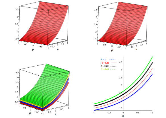
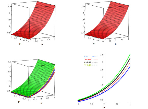
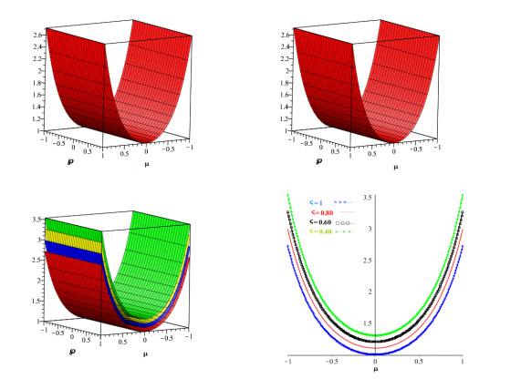
The major goal of this research is to use a new integral transform approach to obtain the exact solution to the time-fractional convection-reaction-diffusion equations (CRDEs). The proposed method is a combination of the Elzaki transform and the homotopy perturbation method. He's polynomial is used to tackle the nonlinearity which arise in our considered problems.Three test examples are considered to show the accuracy of the proposed scheme. In order to find satisfactory approximations to the offered problems, this work takes into account a sophisticated methodology and fractional operators in this context. In order to achieve better approximations after a limited number of iterations, we first construct the Elzaki transforms of the Caputo fractional derivative (CFD) and Atangana-Baleanu fractional derivative (ABFD) and implement them for CRDEs. It has been found that the proposed method's solution converges at the desired rate towards the accurate solution. We give some graphical representations of the accurate and analytical results, which are in excellent agreement with one another, to demonstrate the validity of the suggested methodology. For validity of the present technique, the convergence of the fractional solutions towards integer order solution is investigated. The proposed method is found to be very efficient, simple, and suitable to other nonlinear problem raised in science and engineering.

Keywords:

Citation: Muhammed Naeem, Noufe H. Aljahdaly, Rasool Shah, Wajaree Weera. The study of fractional-order convection-reaction-diffusion equation via an Elzake Atangana-Baleanu operator[J]. AIMS Mathematics, 2022, 7(10): 18080-18098. doi: 10.3934/math.2022995

Related Papers:

[1]	Yumei Chen, Jiajie Zhang, Chao Pan . Numerical approximation of a variable-order time fractional advection-reaction-diffusion model via shifted Gegenbauer polynomials. AIMS Mathematics, 2022, 7(8): 15612-15632. doi: 10.3934/math.2022855
[2]	Aslı Alkan, Halil Anaç . A new study on the Newell-Whitehead-Segel equation with Caputo-Fabrizio fractional derivative. AIMS Mathematics, 2024, 9(10): 27979-27997. doi: 10.3934/math.20241358
[3]	Muhammad Farman, Ali Akgül, Kottakkaran Sooppy Nisar, Dilshad Ahmad, Aqeel Ahmad, Sarfaraz Kamangar, C Ahamed Saleel . Epidemiological analysis of fractional order COVID-19 model with Mittag-Leffler kernel. AIMS Mathematics, 2022, 7(1): 756-783. doi: 10.3934/math.2022046
[4]	Changdev P. Jadhav, Tanisha B. Dale, Vaijanath L. Chinchane, Asha B. Nale, Sabri T. M. Thabet, Imed Kedim, Miguel Vivas-Cortez . On solutions of fractional differential equations for the mechanical oscillations by using the Laplace transform. AIMS Mathematics, 2024, 9(11): 32629-32645. doi: 10.3934/math.20241562
[5]	Rehana Ashraf, Saima Rashid, Fahd Jarad, Ali Althobaiti . Numerical solutions of fuzzy equal width models via generalized fuzzy fractional derivative operators. AIMS Mathematics, 2022, 7(2): 2695-2728. doi: 10.3934/math.2022152
[6]	Mohammed A. Almalahi, Satish K. Panchal, Fahd Jarad, Mohammed S. Abdo, Kamal Shah, Thabet Abdeljawad . Qualitative analysis of a fuzzy Volterra-Fredholm integrodifferential equation with an Atangana-Baleanu fractional derivative. AIMS Mathematics, 2022, 7(9): 15994-16016. doi: 10.3934/math.2022876
[7]	Fatmawati, Muhammad Altaf Khan, Ebenezer Bonyah, Zakia Hammouch, Endrik Mifta Shaiful . A mathematical model of tuberculosis (TB) transmission with children and adults groups: A fractional model. AIMS Mathematics, 2020, 5(4): 2813-2842. doi: 10.3934/math.2020181
[8]	Muhammad Imran Asjad, Waqas Ali Faridi, Adil Jhangeer, Maryam Aleem, Abdullahi Yusuf, Ali S. Alshomrani, Dumitru Baleanu . Nonlinear wave train in an inhomogeneous medium with the fractional theory in a plane self-focusing. AIMS Mathematics, 2022, 7(5): 8290-8313. doi: 10.3934/math.2022462
[9]	Manal Alqhtani, Khaled M. Saad, Rasool Shah, Thongchai Botmart, Waleed M. Hamanah . Evaluation of fractional-order equal width equations with the exponential-decay kernel. AIMS Mathematics, 2022, 7(9): 17236-17251. doi: 10.3934/math.2022949
[10]	Saima Rashid, Sobia Sultana, Bushra Kanwal, Fahd Jarad, Aasma Khalid . Fuzzy fractional estimates of Swift-Hohenberg model obtained using the Atangana-Baleanu fractional derivative operator. AIMS Mathematics, 2022, 7(9): 16067-16101. doi: 10.3934/math.2022880

Abstract

1. Introduction

Leibnitz developed a fraction in derivative, revealing that fractional calculus is better suited to modelling real-world problems than classical calculus. Fractional calculus theory provides an effective and systematic interpretation of nature's reality ^[1,2,3]. It has recently attracted interest because to its ability to provide accurate explanations for nonlinear complex systems. Fluid dynamics ^[4], electrodynamics ^[5], nanotechnology, finance, neurophysiology ^[6], and other fields have given fractional-order derivatives increasing attention. The concept of fractional calculus and its applications has developed fast in recent years ^[7,8,9,10]. Fractional calculus, which deals with arbitrary order derivatives and integrals ^[11], is important in many areas of applied science and engineering ^[12,13,14].

Because of its wide applications in the fields of physics and engineering, fractional differential equations have attracted a lot of attention in recent years ^[15]. Fractional differential equations accumulate the entire information of the function in a weighted form, as opposed to integer order differential equations, in which derivatives depend only on the local behaviour of the function. The memory effect ^[11,15] has numerous applications in physics, chemistry, and engineering. The solution of fractional order differential equations is a complex task. Due to their precise description of nonlinear phenomena, fractional differential equations have recently received a lot of interest. The broad applicability of these equations is the main reason for their popularity among mathematicians and physicists. Many mathematical models in mathematical biology, aerodynamics, rheology, diffusion, electrostatics, electrodynamics, control theory, fluid mechanics, analytical chemistry, and other fields have recently been successfully applied using nonlinear partial differential equations with fractional order derivatives.

It is essential to get correct or approximate solutions of nonlinear fractional partial differential equations in all of these scientific domains (NFPDEs). However, there is no approach that provides a precise solution for NFPDEs, and the majority of the solutions produced are simply approximations. In mathematical physics, engineering, and other sciences, the study of analytical or numerical solutions to NFDEs is essential. As a result, finding effective and appropriate solutions is essential. To solve NFPDEs, many analytical and numerical methods have been presented. Variational iteration approach ^[16], modified Adomian decomposition method (MADM) ^[17], differential transformation method (DTM) ^[18], optimal homotopy asymptotic method (OHAM) ^[19], and homotopy perturbation transform method (HPTM) ^[20] are the most widely used ones.

Numerous analytical techniques, like generalized Taylor fractional series method ^[21] and Finite difference method ^[22] have been implemented to solve CRDEs. Ali Khalouta used Aboodh variational iteration method to to find the exact solution of CRDEs ^[23]. Şuayip Toprakseven ^[24] used a weak Galerkin finite element method to solve CRDEs. Recently, Mounirah Areshi et al. the iterative transformation method and homotopy perturbation transform method to obtain the solution of CRDEs ^[25] and some other work are as ^[26,27]. In this paper we will suggest the Elzaki transform in combination with the CFD and ABC operators to solve three special CRDEs problems. We consider time-fractional convection-reaction-diffusion equation of the following

$\begin{equation} D_{\wp}^{\varsigma}{\varphi}(\mu, \wp) = \varphi_{{\mu}{\mu}}(\mu, \wp)+\varphi(\mu, \wp)+\varphi(\mu, \wp)\varphi_{{\mu}}(\mu, \wp)-\varphi^{2}(\mu, \wp) \end{equation}$

(1.1)

having initial source

$\begin{equation} \varphi({\mu}, 0) = 1+e^{{\mu}} \end{equation}$

(1.2)

and

$\begin{equation} D_{\wp}^{\varsigma}\varphi(\mu, \wp) = \varphi_{{\mu}{\mu}}(\mu, \wp)-\varphi_{{\mu}}(\mu, \wp)+\varphi(\mu, \wp)+\varphi(\mu, \wp)\varphi_{{\mu}}(\mu, \wp)-\varphi^{2}(\mu, \wp) \end{equation}$

(1.3)

having initial source

$\begin{equation} \varphi({\mu}, 0) = e^{{\mu}} \end{equation}$

(1.4)

and

$\begin{equation} D_{\wp}^{\varsigma}\varphi(\mu, \wp) = \varphi_{{\mu}{\mu}}(\mu, \wp)-(1+4\mu^{2})\varphi(\mu, \wp) \end{equation}$

(1.5)

having initial source

$\begin{equation} \varphi({\mu}, 0) = e^{{\mu}^{2}}. \end{equation}$

(1.6)

In applied sciences, convection-reaction-diffusion problems are very helpful mathematical models. Equations of this type are used to model a variety of phenomena. The convection-reaction-diffusion equation, for example, is used to estimate river water quality by measuring the amount of organic matter contained ^[28]. Measurements of biologic oxygen demand on a section of the river are used to assess the location and intensity of pollution sources. An approach based on the minimization of a Kohn and Vogelius type cost function is used to tackle this inverse problem. In the case of air pollution, similar problems can be investigated ^[29]. Convection-reaction-diffusion equations have also been used to represent a variety of real-world processes, including heat conduction, chemical reaction-diffusion, and cancer tumour growth ^[30].

The following is a description of the paper's structure. We provide some necessary definitions and properties of fractional calculus theory in Section 2. The proposed method to solve CRDEs is introduced in Section 3 using a general methodology. Three examples are shown in Section 4 to demonstrate the efficiency and efficacy of the suggested approach. We present our results in the form of graphs and tables. The conclusion of this research is presented in Section 5.

2. Preliminaries

Here we discuss the basic ideas of fractional calculus and Elzaki transform.

Definition 2.1. The fractional derivative in Caputo manner (CFD) is stated as ^[11]:

$\begin{equation} ^{C}_{0}D_{\wp}^{\varsigma}(\ell(\wp)) = \begin{cases} &\frac{1}{\Gamma(m-\varsigma)}\int_{0}^{\wp} \frac{\ell^{m}(\eta)}{(\wp-\eta)^{\varsigma+1-m}}d\eta, \ \ m-1 < \varsigma < m, \\ &\frac{d^{m}}{d\wp^{m}}\ell(\wp), \ \ \ \ \ \ \ \ \ \ \ \ \ \ \ \ \ \ \ \ \ \ \ \ \ \ \ \varsigma = m. \end{cases} \end{equation}$

(2.1)

Definition 2.2. For a function $\ell(\wp)$ , the Riemann-Liouville integral of order fraction is stated as ^[31,32]

$\begin{equation} \begin{split} I^{{{\rho}}}\ell(\wp) = &\frac{1}{\Gamma({{\varsigma}})}\int_{0}^{\wp}(\wp-\eta)^{{{\varsigma}}-1}\ell(\eta)d\eta, \ \ {{\varsigma}} > 0, \ \ \wp > 0, \\ and \ \ I^{0}\ell(\wp) = &\ell(\wp). \end{split} \end{equation}$

(2.2)

Definition 2.3. The fractional derivative in Atangana-Baleanu Caputo sense (ABC) is stated as ^[33]:

$\begin{equation} ^{ABC}_{m}D_{\wp}^{\varsigma}(\ell(\wp)) = \frac{N(\varsigma)}{1-\varsigma}\int_{m}^{\wp}\ell^{'}(\eta)E_{\varsigma}\left[-\frac{\varsigma(\wp-\eta)^{\varsigma}}{1-\varsigma}\right]d\eta, \end{equation}$

(2.3)

where $\ell\in H^{1}(\alpha, \beta), \beta > \alpha, \varsigma\in[0, 1]$ . When $\varsigma = 0$ and $\varsigma = 1$ then normalisation function equal to $1$ and is denoted by $N(\varsigma)$ as given in Eq (2.3).

Definition 2.4. The integral having fractional-order of ABC operator is stated as ^[33]

$\begin{equation} ^{ABC}_{m}I_{\wp}^{\varsigma}(\ell(\wp)) = \frac{1-\varsigma}{N(\varsigma)}\ell(\wp)+\frac{\varsigma}{\Gamma(\varsigma)N(\varsigma)}\int_{m}^{\wp}\ell(\eta)(\wp-\eta)^{\varsigma-1}d\eta. \end{equation}$

(2.4)

Definition 2.5. For exponential function, the Elzaki transform's is stated as in set $A$ ^[34]

$\begin{equation} A = \{\ell(\wp):\exists G, p_{1}, p_{2} > 0, |\ell(\wp)| < Ge^{\frac{|\wp|}{p_{j}}}, if \ \ \wp\in(-1)^{j}\times[0, \infty)\}. \end{equation}$

(2.5)

In the set, $G$ is a finite number for a certain function, but $p_{1}$ , $p_{2}$ may be finite or infinite.

Definition 2.6. The Elzaki transform is stated as ^[35,36]

$\begin{equation} \mathcal{E}\left\{\ell(\wp)\right\}(\varpi) = \tilde{U}(\varpi) = \varpi\int_{0}^{\infty}e^{-\frac{\wp}{\varpi}}\ell(\wp)d\wp, \end{equation}$

(2.6)

where $\wp\geq0, p_{1}\leq\varpi\leq p_{2}$ .

Theorem 2.7. (Convolution theorem, ^[37]) The given equality holds:

$\begin{equation} \mathcal{E}\{\ell*v\} = \frac{1}{\varpi}\mathcal{E}(\ell)\mathcal{E}(v), \end{equation}$

(2.7)

where $\mathcal{E}\{.\}$ represents the Elzaki transform.

Definition 2.8. For the CFD operator $^{C}_{0}D^{\varsigma}_{\wp}(\ell(\wp))$ , the Elzaki transform is stated as ^[38]

$\begin{equation} \mathcal{E}\{^{C}_{0}D_{\wp}^{\varsigma}(\ell(\wp))\}(\varpi) = \varpi^{-\varsigma}\tilde{U}(\varpi)-\sum\limits_{k = 0}^{m-1}\varpi^{2-\varsigma+k}\ell^{k}(0), \end{equation}$

(2.8)

where $m-1 < \varsigma < m$ .

Theorem 2.9. The Elzaki transform in terms of fractional ABC derivative $^{ABC}_{m}D^{\varsigma}_{\wp}(\ell(\wp))$ is stated as

$\begin{equation} \mathcal{E}\{^{ABC}_{m}D_{\wp}^{\varsigma}(\ell(\wp))\}(\varpi) = \frac{N(\varsigma)\varpi}{\varsigma\varpi^{\varsigma}+1-\varsigma}\left(\frac{\tilde{U}(\varpi)}{\varpi}-\varpi \ell(0)\right), \end{equation}$

(2.9)

where $\mathcal{E}\{\ell(\wp)\}\varpi = \tilde{U}(\varpi)$ .

Proof. As we know by Definition 2.3, thus:

$\begin{equation} \mathcal{E}\{^{ABC}_{m}D_{\wp}^{\varsigma}(\ell(\wp))\}(\varpi) = \mathcal{E}\left\{\frac{N(\varsigma)}{1-\varsigma}\int_{0}^{\wp}\ell^{'}(\eta)E_{\varsigma}\left[-\frac{\varsigma(\wp-\eta)^{\varsigma}}{1-\varsigma}\right]d\eta\right\}(\varpi). \end{equation}$

(2.10)

Hence by the definition and and convolution of the Elzaki transform, we have

$\begin{equation} \begin{split} \mathcal{E}\{^{ABC}_{m}D_{\wp}^{\varsigma}(\ell(\wp))\}(\varpi) = &\mathcal{E}\left\{\frac{N(\varsigma)}{1-\varsigma}\int_{0}^{\wp}\ell^{'}(\eta)E_{\varsigma}\left[-\frac{\varsigma(\wp-\eta)^{\varsigma}}{1-\varsigma}\right]d\eta\right\}\\ = &\frac{N(\varsigma)}{1-\varsigma}\frac{1}{\varpi}\mathcal{E}\left\{\ell^{'}(\eta)\right\}\mathcal{E}\left\{E_{\varsigma}\left[-\frac{\varsigma\wp^{\varsigma}}{1-\varsigma}\right]d\eta\right\}\\ = &\frac{N(\varsigma)}{1-\varsigma}\left[\frac{\tilde{U}(\varpi)}{\varpi}-\varpi \ell(0)\right]\left[\int_{0}^{\infty}e^{-\frac{1}{\varpi}}E_{\varsigma}\left[-\frac{\varsigma\wp^{\varsigma}}{1-\varsigma}\right]d\wp\right]\\ = &\frac{N(\varsigma)\varpi}{\varsigma\varpi^{\varsigma}+1-\varsigma}\left[\frac{\tilde{U}(\varpi)}{\varpi}-\varpi \ell(0)\right]. \end{split} \end{equation}$

(2.11)

3. General methodology

This section of the study will cover the most important technique used in this investigation. To explore this methodology, we utilise the fractional nonlinear PDE general form:

$\begin{equation} \begin{split} &D_{\wp}^{\varsigma}\varphi(\mu, \wp)+L(\varphi(\mu, \wp))+N(\varphi(\mu, \wp)) = \theta(\mu, \wp), \\ &(\mu, \wp)\in[0, 1]\times[0, T], \ \ \kappa-1 < \varsigma < \kappa, \end{split} \end{equation}$

(3.1)

with initial source

$\begin{equation} \frac{\partial^{z}\varphi}{\partial \wp^{z}}(\mu, 0) = \ell_{z}(\mu), \ \ z = 0, 1, \cdots, \kappa-1, \end{equation}$

(3.2)

and the boundary conditions

$\begin{equation} \varphi(0, \wp) = \gamma_{0}(\wp), \ \ \varphi(\mu, \wp) = \gamma_{1}(\wp), \ \ \wp\geq0, \end{equation}$

(3.3)

where known functions are $\ell_{z}, \theta, \gamma_{0}$ , and $\gamma_{1}$ . In Eq (3.1), the Caputo or ABC fractional derivatives are represented by $D_{\wp}^{\varsigma}\varphi(\mu, \wp)$ while the linear and non linear terms are denoted by $L(.)$ and $N(.)$ . We study $E\{\varphi(\mu, \wp)\}(\varpi) = \tilde{\zeta}(\mu, \varpi)$ for Eq (3.1) by using CFD in Eq (2.8) and ABC in Eq (2.9) to perform the Elzaki transform. The fractional Caputo derivative's modified functions can then be obtained.

$\begin{equation} \tilde{\zeta}(\mu, \varpi) = \varpi^{\varsigma}(\tilde{\theta}({\varpi}, \wp)-\mathcal{E}[L(\varphi(\mu, \wp))+N(\varphi(\mu, \wp))])+\varpi^{2}\varphi(\mu, 0). \end{equation}$

(3.4)

We also acquire the ABC derivative's modified functions, which are as follows:

$\begin{equation} \tilde{\zeta}(\mu, \varpi) = \left(\frac{\varsigma\varpi^{\varsigma}+1-\varsigma}{N(\varsigma)}\right)(\tilde{\theta}(\mu, \varpi)-\mathcal{E}[L(\varphi(\mu, \wp))+N(\varphi(\mu, \wp))])+\varpi^{2}\varphi(\mu, 0), \end{equation}$

(3.5)

where $\mathcal{E}[\theta(\mu, \wp)] = \tilde{\theta}(\mu, \varpi)$ . Now by taking the Elzaki transform of the boundary conditions, have.

$\begin{equation} \mathcal{E}[\gamma_{0}(\wp)] = \tilde{\zeta}(0, \varpi), \ \ \mathcal{E}[\gamma_{1}(\wp)] = \tilde{\zeta}(1, \varpi), \ \ \varpi\geq0. \end{equation}$

(3.6)

The perturbation approach is then used to derive the solution to Eqs (3.1)–(3.3)

$\begin{equation} \tilde{\zeta}(\mu, \varpi) = \sum\limits_{\mathcal{E} = 0}^{\infty}\mathcal{X}^{\mathcal{E}}\tilde{\zeta}_{\mathcal{E}}(\mu, \varpi), \ \ \mathcal{E} = 0, 1, 2, \cdots \end{equation}$

(3.7)

The nonlinear component in Eq (3.1) can be derived as

$\begin{equation} N[\varphi(\mu, \wp)] = \sum\limits_{\mathcal{E} = 0}^{\infty}\mathcal{X}^{\mathcal{E}}\mu_{\mathcal{E}}(\mu, \wp), \end{equation}$

(3.8)

and the parts $\mu_{\mathcal{E}}(\mu, \wp)$ are define as

$\begin{equation} \mu_{\mathcal{E}}(\varphi_{0}, \varphi_{1}, \cdots, \varphi_{\mathcal{E}}) = \frac{1}{\mathcal{E}!}\frac{\partial^{\mathcal{E}}}{\partial \nu^{\mathcal{E}}}\left[N\left(\sum\limits_{i = 0}^{\infty}\nu^{i}\varphi_{i}\right)\right]_{\nu = 0}, \ \ \mathcal{E} = 0, 1, 2, \cdots \end{equation}$

(3.9)

We get the components of the Caputo operator's solution by substituting Eqs (3.7) and (3.8) into Eq (3.4),

$\begin{equation} \begin{split} \sum\limits_{\mathcal{E} = 0}^{\infty}\mathcal{X}^{\mathcal{E}}\tilde{\zeta}(\mu, \varpi) = &-\mathcal{X}\varpi^{\varsigma}\left(\mathcal{E}\left[L\left(\sum\limits_{\mathcal{E} = 0}^{\infty}\mathcal{X}^{\mathcal{E}}\varphi_{\mathcal{E}}(\mu, \wp)\right)+\sum\limits_{\mathcal{E} = 0}^{\infty}\mathcal{X}^{\mathcal{E}}\mu_{\mathcal{E}}(\mu, \wp)\right]\right)\\ &+\varpi^{\varsigma}(\tilde{\theta}(\mu, \varpi))+\varpi^{2}\varphi(\mu, 0). \end{split} \end{equation}$

(3.10)

We possess the recursive relation that results in the solution of the Atangana-Baleanu operator by sustituting Eqs (3.7) and (3.8) into Eq (3.5),

$\begin{equation} \begin{split} \sum\limits_{\mathcal{E} = 0}^{\infty}\mathcal{X}^{\mathcal{E}}\tilde{\zeta}(\mu, \varpi) = &-\mathcal{X}\left(\frac{\varsigma\varpi^{\varsigma}+1-\varsigma}{N(\varsigma)}\right)\left(\mathcal{E}\left[L\left(\sum\limits_{\mathcal{E} = 0}^{\infty}\mathcal{X}^{\mathcal{E}}\varphi_{\mathcal{E}}(\mu, \wp)\right)+\sum\limits_{\mathcal{E} = 0}^{\infty}\mathcal{X}^{\mathcal{E}}\mu_{\mathcal{E}}(\mu, \wp)\right]\right)\\ &+\left(\frac{\varsigma\varpi^{\varsigma}+1-\varsigma}{N(\varsigma)}\right)(\tilde{\theta}(\mu, \varpi))+\varpi^{2}\varphi(\mu, 0). \end{split} \end{equation}$

(3.11)

Thus, when Eqs (3.10) and (3.11) are solved with regard to $\mathcal{X}$ , the following Caputo homotopies are derived:

$\begin{equation} \begin{split} \mathcal{X}^{0}:\tilde{\zeta}_{0}(\mu, \varpi) = &\varpi^{\varsigma}(\tilde{\theta}(\mu, \varpi))+\varpi^{2}\varphi(\mu, 0), \\ \mathcal{X}^{1}:\tilde{\zeta}_{1}(\mu, \varpi) = &-\varpi^{\varsigma}\mathcal{E}\left[L(\varphi_{0}(\mu, \wp))+\mu_{0}(\mu, \wp)\right], \\ \mathcal{X}^{2}:\tilde{\zeta}_{2}(\mu, \varpi) = &-\varpi^{\varsigma}\mathcal{E}\left[L(\varphi_{1}(\mu, \wp))+\mu_{1}(\mu, \wp)\right], \\ &\vdots\\ \mathcal{X}^{n+1}:\tilde{\zeta}_{n+1}(\mu, \varpi) = &-\varpi^{\varsigma}\mathcal{E}\left[L(\varphi_{n}(\mu, \wp))+\mu_{n}(\mu, \wp)\right]. \end{split} \end{equation}$

(3.12)

Furthermore, the ABC homotopies are determined as follows:

$\begin{equation} \begin{split} \mathcal{X}^{0}:\tilde{\zeta}_{0}(\mu, \varpi) = &\left(\frac{\varsigma\varpi^{\varsigma}+1-\varsigma}{N(\varsigma)}\right)\tilde{\theta}(\mu, \varpi)+\varpi^{2}\varphi(\mu, 0), \\ \mathcal{X}^{1}:\tilde{\zeta}_{1}(\mu, \varpi) = &-\left(\frac{\varsigma\varpi^{\varsigma}+1-\varsigma}{N(\varsigma)}\right)\mathcal{E}\left[L(\varphi_{0}(\mu, \wp))+\mu_{0}(\mu, \wp)\right], \\ \mathcal{X}^{2}:\tilde{\zeta}_{2}(\mu, \varpi) = &-\left(\frac{\varsigma\varpi^{\varsigma}+1-\varsigma}{N(\varsigma)}\right)\mathcal{E}\left[L(\varphi_{1}(\mu, \wp))+\mu_{1}(\mu, \wp)\right], \\ &\vdots\\ \mathcal{X}^{n+1}:\tilde{\zeta}_{n+1}(\mu, \varpi) = &-\left(\frac{\varsigma\varpi^{\varsigma}+1-\varsigma}{N(\varsigma)}\right)\mathcal{E}\left[L(\varphi_{n}(\mu, \wp))+\mu_{n}(\mu, \wp)\right]. \end{split} \end{equation}$

(3.13)

When $\mathcal{X}\rightarrow1$ is used, we can assume that Eqs (3.12) and (3.13) are the approximate solutions to Eqs (3.10) and (3.11), and that the solution is

$\begin{equation} \varsigma_{n}(\mu, \varpi) = \sum\limits_{\varsigma = 0}^{n}\tilde{\zeta}_{\varsigma}(\mu, \varpi). \end{equation}$

(3.14)

By taking the inverse ET to Eq (3.14), we can estimate the solution of Eq (3.1).

$\begin{equation} \varphi(\mu, \varpi)\cong\varphi_{n}(\mu, \wp) = \mathcal{E}^{-1}|\{\varsigma_{n}(\mu, \varpi)\}. \end{equation}$

(3.15)

4. Applications

Example 1. In this part, we'll use the Elzaki transform to look at the problems in Eqs (1.1)–(1.6). To solve problem (1.1) with an initial source, we first use the Elzaki transform technique with the help of the Caputo derivative (1.2). We get by using the Elzaki transform.

$\begin{equation} \tilde{\zeta}(\mu, \varpi) = \varpi^{\varsigma}\mathcal{E}\left[\varphi_{\mu\mu}(\mu, \wp)+\varphi(\mu, \wp)+\varphi(\mu, \wp)\varphi_{\mu}(\mu, \wp)-\varphi^{2}(\mu, \wp)\right]+\varpi^{2}\varphi(\mu, 0). \end{equation}$

(4.1)

To solve Eq (4.1), we employ the Elzaki perturbation transform method

$\sum\limits_{\mathcal{E} = 0}^{\infty}\mathcal{X}^{\mathcal{E}}\tilde{\zeta_{\mathcal{E}}}(\mu, \varpi) = \mathcal{X}\varpi^{\varsigma}\mathcal{E}\left[\left(\sum\limits_{\mathcal{E} = 0}^{\infty}\mathcal{X}^{\mathcal{E}}{\varphi_{\mathcal{E}}}(\mu, \wp)\right)_{\mu\mu}+\left(\sum\limits_{\mathcal{E} = 0}^{\infty}\mathcal{X}^{\mathcal{E}}{\varphi_{\mathcal{E}}}(\mu, \wp)\right)\right]+\\ \mathcal{X}\varpi^{\varsigma}\mathcal{E}\left[\left(\sum\limits_{\mathcal{E} = 0}^{\infty}\mathcal{X}^{\mathcal{E}}\mu_{\mathcal{E}}(\mu, \wp)\right)\right]+\varpi^{2}\varphi(\mu, 0).$

(4.2)

By using the Elzaki inverse transform to Eq (4.2), we now have

$\begin{equation} \begin{split} &\sum\limits_{\mathcal{E} = 0}^{\infty}\mathcal{X}^{\mathcal{E}}{\varphi_{\mathcal{E}}}(\mu, \varpi) = \mathcal{X}\mathcal{E}^{-1}\left[\varpi^{\varsigma}\mathcal{E}\left[\left(\sum\limits_{\mathcal{E} = 0}^{\infty}\mathcal{X}^{\mathcal{E}}{\varphi_{\mathcal{E}}}(\mu, \wp)\right)_{\mu\mu}+\left(\sum\limits_{\mathcal{E} = 0}^{\infty}\mathcal{X}^{\mathcal{E}}{\varphi_{\mathcal{E}}}(\mu, \wp)\right)\right]\right]\\ &+\mathcal{X}\mathcal{E}^{-1}\left[\varpi^{\varsigma}\mathcal{E}\left[\left(\sum\limits_{\mathcal{E} = 0}^{\infty}\mathcal{X}^{\mathcal{E}}\mu_{\mathcal{E}}(\mu, \wp)\right)\right]\right]+\mathcal{E}^{-1}[\varpi^{2}\varphi(\mu, 0)].\\ \end{split} \end{equation}$

(4.3)

In Eq (4.3), the $\mu_{\mathcal{E}}(.)$ represents the nonlinear terms assumed in Eq (3.10),

$\begin{equation} \begin{split} \mu_{0}(\varphi) = &\varphi_{0}(\varphi_{0})_\mu-(\varphi_{0})^{2}, \\ \mu_{1}(\varphi) = &\varphi_{0}(\varphi_{1})_\mu+\varphi_{1}(\varphi_{0})_\mu-2\varphi_{0}\varphi_{1}, \\ \mu_{2}(\varphi) = &\varphi_{0}(\varphi_{2})_\mu+\varphi_{1}(\varphi_{1})_\mu+\varphi_{2}(\varphi_{0})_\mu-2\varphi_{0}\varphi_{2}-(\varphi_{2})^{2}, \\ &\vdots \end{split} \end{equation}$

(4.4)

The terms of the Caputo operator solution are then obtained by evaluating the related powers of $\mathcal{X}$ :

$\begin{equation} \begin{split} \mathcal{X}^{0}:\tilde{\zeta}_{0}(\mu, \wp) = &\mathcal{E}^{-1}[\varpi^{2}1+e^{(\mu)}] = 1+e^{(\mu)}, \\ \mathcal{X}^{1}:\tilde{\zeta}_{1}(\mu, \wp) = &\mathcal{E}^{-1}[\varpi^{\varsigma}\mathcal{E}[L(\varphi_{0}(\mu, \wp))]]+\mathcal{E}^{-1}[\varpi^{\varsigma}\mathcal{E}[\mu_{0}(\mu, \wp)]] = 1+e^{(\mu)}\frac{\wp^{\varsigma}}{\Gamma(\varsigma+1)}, \\ \mathcal{X}^{2}:\tilde{\zeta}_{2}(\mu, \wp) = &\mathcal{E}^{-1}[\varpi^{\varsigma}\mathcal{E}[L(\varphi_{1}(\mu, \wp))]]+\mathcal{E}^{-1}[\varpi^{\varsigma}\mathcal{E}[\mu_{1}(\mu, \wp)]] = 1+e^{(\mu)}\frac{\wp^{2\varsigma}}{\Gamma(2\varsigma+1)}, \\ &\vdots\\ \end{split} \end{equation}$

(4.5)

Thus, we get

$\begin{equation} \begin{split} &\varphi(\mu, \wp) = \Bigg(1+e^{(\mu)}+1+e^{(\mu)}\frac{\wp^{\varsigma}}{\Gamma(\varsigma+1)}+1+e^{(\mu)}\frac{\wp^{2\varsigma}}{\Gamma(2\varsigma+1)}+\cdots\Bigg), \\ \end{split} \end{equation}$

(4.6)

$\begin{equation*} \varphi(\mu, \wp) = 1+e^{(\mu)}\Bigg(1+\frac{\wp^{\varsigma}}{\Gamma(\varsigma+1)}+\frac{\wp^{2\varsigma}}{\Gamma(2\varsigma+1)}+\cdots\Bigg), \end{equation*}$

which provides the problem's integer-order $(\varsigma = 1)$ solution, $\varphi(\mu, \wp) = 1+e^{(\mu+\wp)}$ .

On the other side, we solve the problem using the Elzaki transform in connection with the Atangana-Baleanu operator. To begin, we solve the problem using the Elzaki transform:

$\begin{equation} \tilde{\zeta}(\mu, \varpi) = \left(\frac{\varsigma\varpi^{\varsigma}+1-\varsigma}{N(\varsigma)}\right)\mathcal{E}\left[\varphi_{\mu\mu}(\mu, \wp)+\varphi(\mu, \wp)+\varphi(\mu, \wp)\varphi_{\mu}(\mu, \wp)-\varphi^{2}(\mu, \wp)\right]+\varpi^{2}\varphi(\mu, 0). \end{equation}$

(4.7)

To solve Eq (4.7), we employ the Elzaki perturbation transform method

$\begin{equation} \begin{split} \sum\limits_{\mathcal{E} = 0}^{\infty}\mathcal{X}^{\mathcal{E}}\tilde{\zeta}_{\mathcal{E}}(\mu, \varpi) = &\mathcal{X}\left(\frac{\varsigma\varpi^{\varsigma}+1-\varsigma}{N(\varsigma)}\right)\mathcal{E}\left[\left(\sum\limits_{\mathcal{E} = 0}^{\infty}\mathcal{X}^{\mathcal{E}}{\varphi}_{\mathcal{E}}(\mu, \wp)\right)_{\mu\mu}+\left(\sum\limits_{\mathcal{E} = 0}^{\infty}\mathcal{X}^{\mathcal{E}}{\varphi}_{\mathcal{E}}(\mu, \wp)\right)\right]+\\ &\mathcal{X}\left(\frac{\varsigma\varpi^{\varsigma}+1-\varsigma}{N(\varsigma)}\right)\mathcal{E}\left[\left(\sum\limits_{\mathcal{E} = 0}^{\infty}\mathcal{X}^{\mathcal{E}}\mu_{\mathcal{E}}(\mu, \wp)\right)\right]+\varpi^{2}\varphi(\mu, 0).\\ \end{split} \end{equation}$

(4.8)

By using the Elzaki inverse transform to Eq (4.8), we now have

$\begin{equation} \begin{split} \sum\limits_{\mathcal{E} = 0}^{\infty}\mathcal{X}^{\mathcal{E}}{\varphi}_{\mathcal{E}}(\mu, \wp) = &\mathcal{X}\mathcal{E}^{-1}\left[\left(\frac{\varsigma\varpi^{\varsigma}+1-\varsigma}{N(\varsigma)}\right)\mathcal{E}\left[\left(\sum\limits_{\mathcal{E} = 0}^{\infty}\mathcal{X}^{\mathcal{E}}{\varphi}_{\mathcal{E}}(\mu, \wp)\right)_{\mu\mu}-\left(\sum\limits_{\mathcal{E} = 0}^{\infty}\mathcal{X}^{\mathcal{E}}{\varphi}_{\mathcal{E}}(\mu, \wp)\right)\right]\right]+\\ &\mathcal{X}\mathcal{E}^{-1}\left[\left(\frac{\varsigma\varpi^{\varsigma}+1-\varsigma}{N(\varsigma)}\right)\mathcal{E}\left[\left(\sum\limits_{\mathcal{E} = 0}^{\infty}\mathcal{X}^{\mathcal{E}}\mu_{\mathcal{E}}(\mu, \wp)\right)\right]\right] +\mathcal{E}^{-1}[\varpi^{2}\varphi(\mu, 0)]. \end{split} \end{equation}$

(4.9)

Equation (4.9) contains $\mu_{\mathcal{E}}(.)$ terms, which are nonlinear polynomials specified in Eq (3.9). By repeating the methods for nonlinear polynomials, we obtain:

$\begin{equation} \begin{split} \mathcal{X}^{0}:\varphi_{0}(\mu, \wp) = &\mathcal{E}^{-1}[\varpi^{2}1+e^{(\mu)}] = 1+e^{(\mu)}, \\ \mathcal{X}^{1}:\varphi_{1}(\mu, \wp) = &\mathcal{E}^{-1}[\left(\frac{\varsigma\varpi^{\varsigma}+1-\varsigma}{N(\varsigma)}\right)\mathcal{E}[L(\varphi_{0}(\mu, \wp))]]+\mathcal{E}^{-1}[\left(\frac{\varsigma\varpi^{\varsigma}+1-\varsigma}{N(\varsigma)}\right)\mathcal{E}[\mu_{0}(\mu, \wp)]] = \\ &\Bigg(\frac{1+e^{\mu}}{N(\varsigma)}\Bigg)\left(\frac{\varsigma\wp^{\varsigma}}{\Gamma(\varsigma+1)}+1-\varsigma\right), \\ \mathcal{X}^{2}:\varphi_{2}(\mu, \wp) = &\mathcal{E}^{-1}[\left(\frac{\varsigma\varpi^{\varsigma}+1-\varsigma}{N(\varsigma)}\right)\mathcal{E}[L(\varphi_{1}(\mu, \wp))]]+\mathcal{E}^{-1}[\left(\frac{\varsigma\varpi^{\varsigma}+1-\varsigma}{N(\varsigma)}\right)\mathcal{E}[\mu_{1}(\mu, \wp)]] = \\ &\Bigg(\frac{1+e^{\mu}}{N^{2}(\varsigma)}\Bigg)\left(\frac{(\varsigma\wp^{\varsigma})^{2}}{\Gamma(2\varsigma+1)}+\frac{2\varsigma(1-\varsigma)\wp^{\varsigma}}{\Gamma(\varsigma+1)}+(1-\varsigma)^{2}\right), \\ &\vdots \end{split} \end{equation}$

(4.10)

Hence by means of ABC operator, the obtained solution is as follows:

$\varphi(\mu, \wp) = \sum\limits_{\varsigma = 0}^{n}\varphi_{\varsigma}(\mu, \wp)\\ = 1+e^{\mu}+\frac{1+e^{\mu}}{N(\varsigma)}\left(\frac{\wp^{\varsigma}}{\Gamma(\varsigma)}+1-\varsigma\right)+\frac{1+e^{\mu}}{N^{2}(\varsigma)}\\ \left(\frac{\varsigma^{2}\wp^{2\varsigma}}{\Gamma(2\varsigma+1)}+\frac{(1-\varsigma)\varsigma\wp^{2\varsigma}}{\Gamma(\varsigma+1)}+(1-\varsigma)^{2}\right)+\cdots,$

(4.11)

which provides the problem's integer-order $(\varsigma = 1)$ solution, $\varphi(\mu, \wp) = 1+e^{(\mu+\wp)}$ .

Example 2. Second, to address problem (1.3) with an initial source (1.4), we employ the Elzaki transform technique with the help of the Caputo derivative. We get the following results by applying the Elzaki transform:

$\begin{equation} \tilde{\zeta}(\mu, \varpi) = \varpi^{\varsigma}\mathcal{E}\left[\varphi_{\mu\mu}(\mu, \wp)-\varphi_{\mu}(\mu, \wp)+\varphi(\mu, \wp)+\varphi(\mu, \wp)\varphi_{\mu}(\mu, \wp)-\varphi^{2}(\mu, \wp)\right]+\varpi^{2}\varphi(\mu, 0). \end{equation}$

(4.12)

To solve Eq (4.12), we employ the Elzaki perturbation transform method

$\sum\limits_{\mathcal{E} = 0}^{\infty}\mathcal{X}^{\mathcal{E}}\tilde{\zeta_{\mathcal{E}}}(\mu, \varpi) = \mathcal{X}\varpi^{\varsigma}\mathcal{E}\\ \left[\left(\sum\limits_{\mathcal{E} = 0}^{\infty}\mathcal{X}^{\mathcal{E}}{\varphi_{\mathcal{E}}}(\mu, \wp)\right)_{\mu\mu}+\left(\sum\limits_{\mathcal{E} = 0}^{\infty}\mathcal{X}^{\mathcal{E}}{\varphi_{\mathcal{E}}}(\mu, \wp)\right)-\left(\sum\limits_{\mathcal{E} = 0}^{\infty}\mathcal{X}^{\mathcal{E}}{\varphi_{\mathcal{E}}}(\mu, \wp)\right)_{\mu}\right]+ \\ \mathcal{X}\varpi^{\varsigma}\mathcal{E}\left[\left(\sum\limits_{\mathcal{E} = 0}^{\infty}\mathcal{X}^{\mathcal{E}}\mu_{\mathcal{E}}(\mu, \wp)\right)\right]+\varpi^{2}\varphi(\mu, 0).$

(4.13)

By using the Elzaki inverse transform to Eq (4.13), we now have

$\sum\limits_{\mathcal{E} = 0}^{\infty}\mathcal{X}^{\mathcal{E}}{\varphi_{\mathcal{E}}}(\mu, \varpi) = \mathcal{X}\mathcal{E}^{-1}\\ \left[\varpi^{\varsigma}\mathcal{E}\left[\left(\sum\limits_{\mathcal{E} = 0}^{\infty}\mathcal{X}^{\mathcal{E}}{\varphi_{\mathcal{E}}}(\mu, \wp)\right)_{\mu\mu}+\left(\sum\limits_{\mathcal{E} = 0}^{\infty}\mathcal{X}^{\mathcal{E}}{\varphi_{\mathcal{E}}}(\mu, \wp)\right)-\left(\sum\limits_{\mathcal{E} = 0}^{\infty}\mathcal{X}^{\mathcal{E}}{\varphi_{\mathcal{E}}}(\mu, \wp)\right)_{\mu}\right]\right]\\ +\mathcal{X}\mathcal{E}^{-1}\left[\varpi^{\varsigma}\mathcal{E}\left[\left(\sum\limits_{\mathcal{E} = 0}^{\infty}\mathcal{X}^{\mathcal{E}}\mu_{\mathcal{E}}(\mu, \wp)\right)\right]\right]+\mathcal{E}^{-1}[\varpi^{2}\varphi(\mu, 0)].$

(4.14)

In Eq (4.3), the $\mu_{\mathcal{E}}(.)$ represents the nonlinear terms assumed in Eq (3.10),

(4.15)

The terms of the Caputo operator solution are then obtained by evaluating the related powers of $\mathcal{X}$ :

$\begin{equation} \begin{split} \mathcal{X}^{0}:\tilde{\zeta}_{0}(\mu, \wp) = &\mathcal{E}^{-1}[\varpi^{2}1+e^{(\mu)}] = e^{(\mu)}, \\ \mathcal{X}^{1}:\tilde{\zeta}_{1}(\mu, \wp) = &\mathcal{E}^{-1}[\varpi^{\varsigma}\mathcal{E}[L(\varphi_{0}(\mu, \wp))]]+\mathcal{E}^{-1}[\varpi^{\varsigma}\mathcal{E}[\mu_{0}(\mu, \wp)]] = e^{(\mu)}\frac{\wp^{\varsigma}}{\Gamma(\varsigma+1)}, \\ \mathcal{X}^{2}:\tilde{\zeta}_{2}(\mu, \wp) = &\mathcal{E}^{-1}[\varpi^{\varsigma}\mathcal{E}[L(\varphi_{1}(\mu, \wp))]]+\mathcal{E}^{-1}[\varpi^{\varsigma}\mathcal{E}[\mu_{1}(\mu, \wp)]] = e^{(\mu)}\frac{\wp^{2\varsigma}}{\Gamma(2\varsigma+1)}, \\ &\vdots\\ \end{split} \end{equation}$

(4.16)

Thus, we get

$\begin{equation} \begin{split} &\varphi(\mu, \wp) = \Bigg(e^{(\mu)}+e^{(\mu)}\frac{\wp^{\varsigma}}{\Gamma(\varsigma+1)}+e^{(\mu)}\frac{\wp^{2\varsigma}}{\Gamma(2\varsigma+1)}+\cdots\Bigg), \\ \end{split} \end{equation}$

(4.17)

$\begin{equation*} \varphi(\mu, \wp) = e^{(\mu)}\Bigg(1+\frac{\wp^{\varsigma}}{\Gamma(\varsigma+1)}+\frac{\wp^{2\varsigma}}{\Gamma(2\varsigma+1)}+\cdots\Bigg), \end{equation*}$

which provides the problem's integer-order $(\varsigma = 1)$ solution, $\varphi(\mu, \wp) = e^{(\mu+\wp)}$ .

On the other side, we solve the problem using the Elzaki transform in connection with the Atangana-Baleanu operator. To begin, we solve the problem using the Elzaki transform:

$\begin{equation} \tilde{\zeta}(\mu, \varpi) = \left(\frac{\varsigma\varpi^{\varsigma}+1-\varsigma}{N(\varsigma)}\right)\left(\mathcal{E}\left[\varphi_{\mu\mu}(\mu, \wp)-\varphi_{\mu}(\mu, \wp)+\varphi(\mu, \wp)+\varphi(\mu, \wp)\varphi_{\mu}(\mu, \wp)-\varphi^{2}(\mu, \wp)\right]\right)+\\ \varpi^{2}\varphi(\mu, 0). \end{equation}$

(4.18)

To solve Eq (4.18), we employ the Elzaki perturbation transform method

$\sum\limits_{\mathcal{E} = 0}^{\infty}\mathcal{X}^{\mathcal{E}}\tilde{\zeta}_{\mathcal{E}}(\mu, \varpi) = \mathcal{X}\left(\frac{\varsigma\varpi^{\varsigma}+1-\varsigma}{N(\varsigma)}\right)\mathcal{E}\left\\ [\left(\sum\limits_{\mathcal{E} = 0}^{\infty}\mathcal{X}^{\mathcal{E}}{\varphi}_{\mathcal{E}}(\mu, \wp)\right)_{\mu\mu}+\left(\sum\limits_{\mathcal{E} = 0}^{\infty}\mathcal{X}^{\mathcal{E}}{\varphi}_{\mathcal{E}}(\mu, \wp)\right)-\left(\sum\limits_{\mathcal{E} = 0}^{\infty}\mathcal{X}^{\mathcal{E}}{\varphi}_{\mathcal{E}}(\mu, \wp)\right)_{\mu}\right]+\\ \mathcal{X}\left(\frac{\varsigma\varpi^{\varsigma}+1-\varsigma}{N(\varsigma)}\right)\mathcal{E}\left[\left(\sum\limits_{\mathcal{E} = 0}^{\infty}\mathcal{X}^{\mathcal{E}}\mu_{\mathcal{E}}(\mu, \wp)\right)\right]+\varpi^{2}\varphi(\mu, 0).$

(4.19)

By using the Elzaki inverse transform, we now have

$\sum\limits_{\mathcal{E} = 0}^{\infty}\mathcal{X}^{\mathcal{E}}\tilde{\zeta}_{\mathcal{E}}(\mu, \wp) = \mathcal{X}\mathcal{E}^{-1}\\ \left[\left(\frac{\varsigma\varpi^{\varsigma}+1-\varsigma}{N(\varsigma)}\right)\mathcal{E}\left[\left(\sum\limits_{\mathcal{E} = 0}^{\infty}\mathcal{X}^{\mathcal{E}}{\varphi}_{\mathcal{E}}(\mu, \wp)\right)_{\mu\mu}+\left(\sum\limits_{\mathcal{E} = 0}^{\infty}\mathcal{X}^{\mathcal{E}}{\varphi}_{\mathcal{E}}(\mu, \wp)\right)-\left(\sum\limits_{\mathcal{E} = 0}^{\infty}\mathcal{X}^{\mathcal{E}}{\varphi}_{\mathcal{E}}(\mu, \wp)\right)_{\mu}\right]\right]+\\ \mathcal{X}\mathcal{E}^{-1}\left[\left(\frac{\varsigma\varpi^{\varsigma}+1-\varsigma}{N(\varsigma)}\right)\mathcal{E}\left[\left(\sum\limits_{\mathcal{E} = 0}^{\infty}\mathcal{X}^{\mathcal{E}}\mu_{\mathcal{E}}(\mu, \wp)\right)\right]\right] +\mathcal{E}^{-1}[\varpi^{2}\varphi(\mu, 0)].$

(4.20)

Thus on comparing both sides

$\begin{equation} \begin{split} \mathcal{X}^{0}:\varphi_{0}(\mu, \wp) = &\mathcal{E}^{-1}[\varpi^{2}e^{\mu}] = e^{\mu}, \\ \mathcal{X}^{1}:\varphi_{1}(\mu, \wp) = &\mathcal{E}^{-1}[\left(\frac{\varsigma\varpi^{\varsigma}+1-\varsigma}{N(\varsigma)}\right)\mathcal{E}[L(\varphi_{0}(\mu, \wp))]]+\mathcal{E}^{-1}[\left(\frac{\varsigma\varpi^{\varsigma}+1-\varsigma}{N(\varsigma)}\right)\mathcal{E}[\mu_{0}(\mu, \wp)]] = \\ = &\frac{e^{\mu}}{N(\varsigma)}\left(\frac{\wp^{\varsigma}}{\Gamma(\varsigma)}+1-\varsigma\right), \\ \mathcal{X}^{2}:\varphi_{2}(\mu, \wp) = &\mathcal{E}^{-1}[\left(\frac{\varsigma\varpi^{\varsigma}+1-\varsigma}{N(\varsigma)}\right)\mathcal{E}[L(\varphi_{1}(\mu, \wp))]]+\mathcal{E}^{-1}[\left(\frac{\varsigma\varpi^{\varsigma}+1-\varsigma}{N(\varsigma)}\right)\mathcal{E}[\mu_{1}(\mu, \wp)]] = \\ = &\frac{e^{\mu}}{N^{2}(\varsigma)}\left(\frac{\varsigma^{2}\wp^{2\varsigma}}{\Gamma(2\varsigma+1)}+\frac{(1-\varsigma)\varsigma\wp^{2\varsigma}}{\Gamma(\varsigma+1)}+(1-\varsigma)^{2}\right)\\ \end{split} \end{equation}$

(4.21)

Hence by means of ABC operator, the obtained solution is as follows:

$\begin{equation} \varphi(\mu, \wp) = e^{\mu}+\frac{e^{\mu}}{N(\varsigma)}\left(\frac{\wp^{\varsigma}}{\Gamma(\varsigma)}+1-\varsigma\right)+\frac{e^{\mu}}{N^{2}(\varsigma)}\left(\frac{\varsigma^{2}\wp^{2\varsigma}}{\Gamma(2\varsigma+1)}+\frac{(1-\varsigma)\varsigma\wp^{2\varsigma}}{\Gamma(\varsigma+1)}+(1-\varsigma)^{2}\right)+\cdots, \end{equation}$

(4.22)

which provides the problem's integer-order $(\varsigma = 1)$ solution, $\varphi(\mu, \wp) = e^{(\wp+\mu)}$ .

Example 3. Finally, to address problem (1.5) with an initial source (1.6), we employ the Elzaki transform technique with the help of the Caputo and ABC derivative. To Eqs (1.5) and (1.6), we first employ the Elzaki transform along with the aid of Caputo derivative:

$\begin{equation} \tilde{\zeta}(\mu, \varpi) = \varpi^{\varsigma}\mathcal{E}\left[\varphi_{\mu\mu}(\mu, \wp)-(1+4\mu^{2})\varphi(\mu, \wp)\right]+\varpi^{2}\varphi(\mu, 0). \end{equation}$

(4.23)

To solve Eq (4.23), we employ the Elzaki perturbation transform method

$\sum\limits_{\mathcal{E} = 0}^{\infty}\mathcal{X}^{\mathcal{E}}\tilde{\zeta}_{\mathcal{E}}(\mu, \varpi) = \mathcal{X}\varpi^{\varsigma}\mathcal{E}\left[\left(\sum\limits_{\mathcal{E} = 0}^{\infty}\mathcal{X}^{\mathcal{E}}{\varphi}_{\mathcal{E}}(\mu, \varpi)\right)_{\mu\mu}-(1+4\mu^{2})\left(\sum\limits_{\mathcal{E} = 0}^{\infty}\mathcal{X}^{\mathcal{E}}{\varphi}_{\mathcal{E}}(\mu, \varpi)\right)\right]+\\ \varpi^{2}\varphi(\mu, 0).$

(4.24)

By using the Elzaki inverse transform to Eq (4.24), we now have

$\sum\limits_{\mathcal{E} = 0}^{\infty}\mathcal{X}^{\mathcal{E}}{\varphi}_{\mathcal{E}}(\mu, \wp) = \mathcal{X}\mathcal{E}^{-1}\left[\varpi^{\varsigma}\mathcal{E}\left[\left(\sum\limits_{\mathcal{E} = 0}^{\infty}\mathcal{X}^{\mathcal{E}}{\varphi}_{\mathcal{E}}(\mu, \wp)\right)-(1+4\mu^{2})\left(\sum\limits_{\mathcal{E} = 0}^{\infty}\mathcal{X}^{\mathcal{E}}{\varphi}_{\mathcal{E}}(\mu, \varpi)\right)\right]\right]\\ +\mathcal{E}^{-1}\left[\varpi^{2}\varphi(\mu, 0)\right].$

(4.25)

The terms of the Caputo operator solution are then obtained by evaluating the related powers of $\mathcal{X}$ :

$\begin{equation} \begin{split} \mathcal{X}^{0}:\varphi_{0}(\mu, \wp) = &\mathcal{E}^{-1}[\varpi^{2}e^{\mu^{2}}] = e^{\mu^{2}}, \\ \mathcal{X}^{1}:\varphi_{1}(\mu, \wp) = &\mathcal{E}^{-1}[\varpi^{\varsigma}\mathcal{E}[L(\varphi_{0}(\mu, \wp))]], \\ = &e^{\mu^{2}}\frac{\wp^{\varsigma}}{\Gamma(\varsigma+1)}, \\ \mathcal{X}^{2}:\varphi_{1}(\mu, \wp) = &\mathcal{E}^{-1}[\varpi^{\varsigma}\mathcal{E}[L(\varphi_{1}(\mu, \wp))]], \\ = &e^{\mu^{2}}\frac{\wp^{2\varsigma}}{\Gamma(2\varsigma+1)}, \\ &\vdots \end{split} \end{equation}$

(4.26)

Thus, we get

$\begin{equation} \varphi(\mu, \wp) = e^{\mu^{2}}+e^{\mu^{2}}\frac{\wp^{\varsigma}}{\Gamma(\varsigma+1)}+e^{\mu^{2}}\frac{\wp^{2\varsigma}}{\Gamma(2\varsigma+1)}+\cdots \end{equation}$

(4.27)

which provides the problems integer-order $(\varsigma = 1)$ solution $\varphi(\mu, \wp) = e^{\mu^{2}+\wp}$ .

On the other side, we solve the problem using the Elzaki transform in connection with the Atangana-Baleanu operator. To begin, we solve the problem using the Elzaki transform:

$\begin{equation} \tilde{\zeta}(\mu, \varpi) = \left(\frac{\varsigma\varpi^{\varsigma}+1-\varsigma}{N(\varsigma)}\right)\left(\mathcal{E}\left[\varphi_{\mu\mu}(\mu, \wp)-(1+4\mu^{2})\varphi(\mu, \wp)\right]\right)+\varpi^{2}\varphi(\mu, 0). \end{equation}$

(4.28)

To solve Eq (4.28), we employ the Elzaki perturbation transform method

$\sum\limits_{\mathcal{E} = 0}^{\infty}\mathcal{X}^{\mathcal{E}}\tilde{\zeta}_{\mathcal{E}}(\mu, \varpi) = \left(\frac{\varsigma\varpi^{\varsigma}+1-\varsigma}{N(\varsigma)}\right)\Bigg(\mathcal{E}\left[\left(\sum\limits_{\mathcal{E} = 0}^{\infty}\mathcal{X}^{\mathcal{E}}{\varphi}_{\mathcal{E}}(\mu, \wp)\right)_{\mu\mu}-(1+4\mu^{2})\left(\sum\limits_{\mathcal{E} = 0}^{\infty}\mathcal{X}^{\mathcal{E}}{\varphi}_{\mathcal{E}}(\mu, \wp)\right)\right]\Bigg)\\ +\varpi^{2}\varphi(\mu, 0).$

(4.29)

By using the Elzaki inverse transform, we now have

$\sum\limits_{\mathcal{E} = 0}^{\infty}\mathcal{X}^{\mathcal{E}}{\varphi}_{\mathcal{E}}(\mu, \wp) = \mathcal{X}\mathcal{E}^{-1}\left[\left(\frac{\varsigma\varpi^{\varsigma}+1-\varsigma}{N(\varsigma)}\right)\mathcal{E}\left[\left(\sum\limits_{\mathcal{E} = 0}^{\infty}\mathcal{X}^{\mathcal{E}}\varphi_{\mathcal{E}}(\mu, \wp)\right)-(1+4\mu^{2})\left(\sum\limits_{\mathcal{E} = 0}^{\infty}\mathcal{X}^{\mathcal{E}}{\varphi}_{\mathcal{E}}(\mu, \varpi)\right)\right]\right]\\ +\mathcal{E}^{-1}[\varpi^{2}\varphi(\mu, 0)].$

(4.30)

Thus on comparing both sides

$\begin{equation} \begin{split} \mathcal{X}^{0}:\varphi_{0}(\mu, \wp) = &\mathcal{E}^{-1}[\varpi^{2}\sin\mu] = e^{\mu^{2}}, \\ \mathcal{X}^{1}:\varphi_{1}(\mu, \wp) = &\mathcal{E}^{-1}\left[\left(\frac{\varsigma\varpi^{\varsigma}+1-\varsigma}{N(\varsigma)}\right)\mathcal{E}\left[L(\varphi_{0}(\mu, \wp))\right]\right]\\ = &\frac{e^{\mu^{2}}}{N(\varsigma)}\left(\frac{\wp^{\varsigma}}{\Gamma(\varsigma)}+1-\varsigma\right), \\ \mathcal{X}^{2}:\varphi_{2}(\mu, \wp) = &\mathcal{E}^{-1}\left[\left(\frac{\varsigma\varpi^{\varsigma}+1-\varsigma}{N(\varsigma)}\right)\mathcal{E}\left[L(\varphi_{1}(\mu, \wp))\right]\right]\\ = &\frac{e^{\mu^{2}}}{N^{2}(\varsigma)}\left(\frac{\varsigma^{2}\wp^{2\varsigma}}{\Gamma(2\varsigma+1)}+\frac{(1-\varsigma)\varsigma\wp^{2\varsigma}}{\Gamma(\varsigma+1)}+(1-\varsigma)^{2}\right)\\ \end{split} \end{equation}$

(4.31)

Hence by means of ABC operator, the obtained solution is as follows:

$\begin{equation} \varphi(\mu, \wp) = e^{\mu^{2}}+\frac{e^{\mu^{2}}}{N(\varsigma)}\left(\frac{\wp^{\varsigma}}{\Gamma(\varsigma)}+1-\varsigma\right)+\frac{e^{\mu^{2}}}{N^{2}(\varsigma)}\left(\frac{\varsigma^{2}\wp^{2\varsigma}}{\Gamma(2\varsigma+1)}+\frac{(1-\varsigma)\varsigma\wp^{2\varsigma}}{\Gamma(\varsigma+1)}+(1-\varsigma)^{2}\right)+\cdots, \end{equation}$

(4.32)

which provides the problems integer-order $(\varsigma = 1)$ solution, $\varphi(\mu, \wp) = e^{\mu^{2}+\wp}$ .

5. Results and discussion

The graphs of the exact and approximate solutions are depicted in Figure 1a and b, whereas the nature of the proposed method solution at various fractional-orders is shown in Figure 1c and d for problem 1. Figure 2a and b illustrate the nature of the exact and proposed method solution while Figure 2c and d demonstrates the behavior of the proposed technique at various fractional-orders. Similarly, Figure 3a and b gives the proposed method comparison with the exact solution and Figure 3c and d shows the layout of the suggested technique at different fractional-orders. In addition, we gives the error comparison in terms of two different fractional derivatives with the aid of various fractional derivatives for CRDEs in Tables 1–3. It is clearly observed from the figures and tables that the proposed method solution are in good agreement with the exact solution and converges quickly towards the exact solution. Also from the figures and tables we can conclude that proposed method solution converges towards exact solution as we tends from fractional-orders towards integer-order.

Figure 1. The behavior of the accurate solution, proposed method solution and proposed method solution at different fractional-orders of

$\varsigma$ ,

$y = 0.5$ of problem 1.

DownLoad: Full-Size Img PowerPoint

Figure 2. The behavior of the accurate solution, proposed method solution and proposed method solution at different fractional-orders of

$\varsigma$ ,

$y = 0.5$ of problem 2.

DownLoad: Full-Size Img PowerPoint

Figure 3. The behavior of the accurate solution, proposed method solution and proposed method solution at different fractional-orders of

$\varsigma$ ,

$y = 0.5$ of problem 3.

DownLoad: Full-Size Img PowerPoint

Table 1. Example 1 error comparison at various fractional-order of

$\varsigma$ .

${{\wp}}$	$\mu$	$\varsigma=0.4$	$\varsigma=0.6$	$\varsigma=0.8$	$\varsigma=1(ETM_{CFD})$	$\varsigma=1(ETM_{ABC})$
	0.2	6.6652990000E-03	4.4438650000E-03	2.2224310000E-03	9.9900000000E-07	9.9900000000E-07
	0.4	7.4765770000E-03	4.9847170000E-03	2.4928580000E-03	1.0010000000E-06	1.0010000000E-06
0.1	0.6	8.4674710000E-03	5.6453130000E-03	2.8231550000E-03	9.9900000000E-07	9.9900000000E-07
	0.8	9.6777550000E-03	6.4521680000E-03	3.2265820000E-03	1.0000000000E-06	1.0000000000E-06
	1	1.1155997000E-02	7.4376630000E-03	3.7193290000E-03	9.9900000000E-07	9.9900000000E-07
	0.2	6.6663790000E-03	4.4449190000E-03	2.2234580000E-03	2.0000000000E-06	2.0000000000E-06
	0.4	7.4776670000E-03	4.9857770000E-03	2.4938880000E-03	2.0010000000E-06	2.0010000000E-06
0.2	0.6	8.4685730000E-03	5.6463810000E-03	2.8241890000E-03	1.9990000000E-06	1.9990000000E-06
	0.8	9.6788700000E-03	6.4532450000E-03	3.2276210000E-03	1.9990000000E-06	1.9990000000E-06
	1	1.1157131000E-02	7.4387530000E-03	3.7203740000E-03	2.0000000000E-06	2.0000000000E-06
	0.2	6.6674550000E-03	4.4459700000E-03	2.2244850000E-03	3.0000000000E-06	3.0000000000E-06
	0.4	7.4787510000E-03	4.9868340000E-03	2.4949170000E-03	3.0000000000E-06	3.0000000000E-06
0.3	0.6	8.4696690000E-03	5.6474460000E-03	2.8252230000E-03	2.9990000000E-06	2.9990000000E-06
	0.8	9.6799800000E-03	6.4543200000E-03	3.2286600000E-03	3.0000000000E-06	3.0000000000E-06
	1	1.1158258000E-02	7.4398390000E-03	3.7214190000E-03	3.0000000000E-06	3.0000000000E-06
	0.2	6.6685300000E-03	4.4470180000E-03	2.2255090000E-03	4.0000000000E-06	4.0000000000E-06
	0.4	7.4798360000E-03	4.9878890000E-03	2.4959450000E-03	4.0000000000E-06	4.0000000000E-06
0.4	0.6	8.4707650000E-03	5.6485080000E-03	2.8262540000E-03	3.9990000000E-06	3.9990000000E-06
	0.8	9.6810900000E-03	6.4553910000E-03	3.2296950000E-03	3.9990000000E-06	3.9990000000E-06
	1	1.1159384000E-02	7.4409200000E-03	3.7224590000E-03	3.9990000000E-06	3.9990000000E-06
	0.2	6.6696010000E-03	4.4480680000E-03	2.2265320000E-03	5.0000000000E-06	5.0000000000E-06
	0.4	7.4809150000E-03	4.9889440000E-03	2.4969690000E-03	5.0000000000E-06	5.0000000000E-06
0.5	0.6	8.4718560000E-03	5.6495700000E-03	2.8272820000E-03	5.0000000000E-06	5.0000000000E-06
	0.8	9.6821930000E-03	6.4564620000E-03	3.2307280000E-03	5.0000000000E-06	5.0000000000E-06
	1	1.1160503000E-02	7.4420020000E-03	3.7234970000E-03	4.9990000000E-06	4.9990000000E-06

| Show Table

DownLoad: CSV

Table 2. Example 2 error comparison at various fractional-order of

$\varsigma$ .

${{\wp}}$	$\mu$	$\varsigma=0.4$	$\varsigma=0.6$	$\varsigma=0.8$	$\varsigma=1(ETM_{CFD})$	$\varsigma=1(ETM_{ABC})$
	0.2	3.6674050000E-03	2.4449250000E-03	1.2224550000E-03	7.0000000000E-09	7.0000000000E-09
	0.4	4.4793800000E-03	2.9862390000E-03	1.4931110000E-03	8.0000000000E-09	8.0000000000E-09
0.1	0.6	5.4711270000E-03	3.6474010000E-03	1.8236890000E-03	9.0000000000E-09	9.0000000000E-09
	0.8	6.6824480000E-03	4.4549450000E-03	2.2274590000E-03	1.2000000000E-08	1.2000000000E-08
	1	8.1619620000E-03	5.4412820000E-03	2.7206250000E-03	1.4000000000E-08	1.4000000000E-08
	0.2	3.6700710000E-03	2.4466910000E-03	1.2233250000E-03	2.4000000000E-08	2.4000000000E-08
	0.4	3.6700710000E-03	2.9883960000E-03	1.4941740000E-03	2.9000000000E-08	2.9000000000E-08
0.2	0.6	5.4751020000E-03	13.6500330000E-03	1.8249860000E-03	3.7000000000E-08	3.7000000000E-08
	0.8	6.6873050000E-03	4.4581610000E-03	2.2290440000E-03	4.5000000000E-08	4.5000000000E-08
	1	8.1678930000E-03	5.4452100000E-03	2.7225600000E-03	5.5000000000E-08	5.5000000000E-08
	0.2	3.6725270000E-03	2.4483130000E-03	1.2241190000E-03	5.5000000000E-08	5.5000000000E-08
	0.4	4.4856350000E-03	2.9903770000E-03	1.4951430000E-03	6.7000000000E-08	6.7000000000E-08
0.3	0.6	5.4787660000E-03	3.6524530000E-03	1.8261710000E-03	8.2000000000E-08	8.2000000000E-08
	0.8	6.6917800000E-03	4.4611160000E-03	2.2304900000E-03	1.0100000000E-07	1.0100000000E-07
	1	8.1733600000E-03	5.4488200000E-03	2.7243270000E-03	1.2200000000E-07	1.2200000000E-07
	0.2	3.6748440000E-03	2.4498380000E-03	1.2248580000E-03	9.8000000000E-08	9.8000000000E-08
	0.4	4.4884650000E-03	2.9922400000E-03	1.4960450000E-03	1.1900000000E-07	1.1900000000E-07
0.4	0.6	5.4822230000E-03	3.6547290000E-03	1.8272730000E-03	1.4600000000E-07	1.4600000000E-07
	0.8	6.6960020000E-03	4.4638960000E-03	2.2318360000E-03	1.7900000000E-07	1.7900000000E-07
	1	8.1785150000E-03	5.4522150000E-03	2.7259710000E-03	2.1800000000E-07	2.1800000000E-07
	0.2	3.6770560000E-03	2.4512910000E-03	1.2255540000E-03	1.5300000000E-07	1.5300000000E-07
	0.4	4.4911670000E-03	2.9940140000E-03	1.4968960000E-03	1.8600000000E-07	1.8600000000E-07
0.5	0.6	5.4855220000E-03	3.6568950000E-03	1.8283110000E-03	2.2900000000E-07	2.2900000000E-07
	0.8	6.7000330000E-03	4.4665420000E-03	2.2331050000E-03	2.7900000000E-07	2.7900000000E-07
	1	8.1834390000E-03	5.4554470000E-03	2.7275210000E-03	3.4000000000E-07	3.4000000000E-07

| Show Table

DownLoad: CSV

Table 3. Example 3 error comparison at various fractional-order of

$\varsigma$ .

${{\wp}}$	$\mu$	$\varsigma=0.4$	$\varsigma=0.6$	$\varsigma=0.8$	$\varsigma=1(ETM_{CFD})$	$\varsigma=1(ETM_{ABC})$
	0.2	3.1251570000E-03	2.0834290000E-03	1.0417080000E-03	5.0000000000E-09	5.0000000000E-09
	0.4	3.5236050000E-03	2.3490590000E-03	1.1745220000E-03	6.0000000000E-09	6.0000000000E-09
0.1	0.6	4.3037410000E-03	2.8691470000E-03	1.4345650000E-03	7.0000000000E-09	7.0000000000E-09
	0.8	5.6944070000E-03	3.7962540000E-03	1.8981150000E-03	1.0000000000E-08	1.0000000000E-08
	1	8.1619620000E-03	5.4412820000E-03	2.7206250000E-03	1.4000000000E-08	1.4000000000E-08
	0.2	3.1274280000E-03	2.0849320000E-03	1.0424490000E-03	2.1000000000E-08	2.1000000000E-08
	0.4	3.5261650000E-03	2.3507540000E-03	1.1753580000E-03	2.4000000000E-08	2.4000000000E-08
0.2	0.6	4.3068690000E-03	2.8712190000E-03	1.4355860000E-03	2.8000000000E-08	2.8000000000E-08
	0.8	5.6985460000E-03	3.7989950000E-03	1.8994660000E-03	3.8000000000E-08	3.8000000000E-08
	1	8.1678930000E-03	5.4452100000E-03	2.7225600000E-03	5.5000000000E-08	5.5000000000E-08
	0.2	3.1295210000E-03	2.0863150000E-03	1.0431260000E-03	4.7000000000E-08	4.7000000000E-08
	0.4	3.5285250000E-03	2.3523130000E-03	1.1761210000E-03	5.3000000000E-08	5.3000000000E-08
0.3	0.6	4.3097510000E-03	2.8731220000E-03	1.4365170000E-03	6.4000000000E-08	6.4000000000E-08
	0.8	5.7023590000E-03	3.8015130000E-03	1.9006980000E-03	8.6000000000E-08	8.6000000000E-08
	1	8.1733600000E-03	5.4488200000E-03	2.7243270000E-03	1.2200000000E-07	1.2200000000E-07
	0.2	3.1314950000E-03	2.0876140000E-03	1.0437550000E-03	8.4000000000E-08	8.4000000000E-08
	0.4	3.5307520000E-03	2.3537790000E-03	1.1768310000E-03	9.4000000000E-08	9.4000000000E-08
0.4	0.6	4.3124700000E-03	2.8749120000E-03	1.4373850000E-03	1.1400000000E-07	1.1400000000E-07
	0.8	5.7059570000E-03	3.8038820000E-03	1.9018460000E-03	1.5200000000E-07	1.5200000000E-07
	1	8.1785150000E-03	5.4522150000E-03	2.7259710000E-03	2.1800000000E-07	2.1800000000E-07
	0.2	3.1333800000E-03	2.0888520000E-03	1.0443480000E-03	1.3100000000E-07	1.3100000000E-07
	0.4	3.5328770000E-03	2.3551740000E-03	1.1775000000E-03	1.4700000000E-07	1.4700000000E-07
0.5	0.6	4.3150660000E-03	2.8766170000E-03	1.4382020000E-03	1.7800000000E-07	1.7800000000E-07
	0.8	5.7093910000E-03	3.8061360000E-03	1.9029270000E-03	2.3800000000E-07	2.3800000000E-07
	1	8.1834390000E-03	5.4554470000E-03	2.7275210000E-03	3.4000000000E-07	3.4000000000E-07

| Show Table

DownLoad: CSV

6. Conclusions

The main concern of this work is to propose an efficient algorithm for the solution of nonlinear fractional convection-diffusion problems. The approximate solutions of some particular time-fractional convection-reaction-diffusion (CRD) equation are found in this paper using a new integral transform technique known as the Elzaki transformation. The proposed approaches are consisted of two steps. The given problems are first simplified using the Elzaki transform, and then the perturbation technique is employed to get the solutions. The proposed method is applied with the aid of two different fractional derivatives named Caputo fractional derivative (CFD) and Atangana-Baleanu fractional derivative (ABFD). The solutions of fractional order problems are investigated and fall into the best representation of the actual dynamics of the problems. To ensure the validity of the proposed method, we showed the results through graphs and tables. The suggested approach main benefit is the series form solution, which quickly converges to the exact solution. The current procedure is found to be very simple and an effective tool for the fractional partial differential equations and therefore can be extended to solve other problems in sciences.

Acknowledgements

The authors would like to thank the Deanship of Scientific Research at Umm Al-Qura University for supporting this work (grant code: 22UQU4310396DSR20).

Conflict of interest

The authors declare that there is no conflict of interest.

References

[1]	J. H. He, A tutorial review on fractal spacetime and fractional calculus, Int. J. Theor. Phys., 53 (2014), 3698–3718. https://doi.org/10.1007/s10773-014-2123-8 doi: 10.1007/s10773-014-2123-8
[2]	F. J. Liu, H. Y. Liu, Z. B. Li, J. H. He, A delayed fractional model for Cocoon heat-proof property, Therm. Sci., 21 (2017), 1867–1871. https://doi.org/10.2298/TSCI160415101L doi: 10.2298/TSCI160415101L
[3]	J. H. He, Fractal calculus and its geometrical explanation, Res. Phys., 10 (2018), 272–276. https://doi.org/10.1016/j.rinp.2018.06.011 doi: 10.1016/j.rinp.2018.06.011
[4]	A. Prakash, P. Veeresha, D. G. Prakasha, M. Goyal, A new efficient technique for solving fractional coupled Navier-Stokes equations using q-homotopy analysis transform method, Pramana, 93 (2019), 6. https://doi.org/10.1007/s12043-019-1763-x doi: 10.1007/s12043-019-1763-x
[5]	V. E. Tarasov, Fractional vector calculus and fractional Maxwell's equations. Ann. Phys., 323 (2008), 2756–2778. https://doi.org/10.1016/j.aop.2008.04.005
[6]	M. Mirzazadeh, A novel approach for solving fractional Fisher equation using differential transform method, Pramana, 86 (2016), 957–963. https://doi.org/10.1007/s12043-015-1117-2 doi: 10.1007/s12043-015-1117-2
[7]	K. Diethelm, N. J. Ford, Analysis of fractional differential equations, J. Math. Anal. Appl., 265 (2002), 229–248. https://doi.org/10.1006/jmaa.2000.7194 doi: 10.1006/jmaa.2000.7194
[8]	K. S. Miller, B. Ross, An introduction to the fractional calculus and fractional differential equations, New York: John Wiley and Sons, 1993.
[9]	F. Mainardi, Fractional calculus: Theory and applications, Mathematics, 6 (2018), 145. https://doi.org/10.3390/math6090145 doi: 10.3390/math6090145
[10]	S. G.Samko, A. A. Kilbas, O. I. Marichev, Fractional integrals and derivatives: Theory and applications, USA: Gordon and breach science publishers, 1993.
[11]	R. W. Ibrahim, Fractional complex transforms for fractional differential equations, Adv. Differ. Equ., 2012 (2012), 192. https://doi.org/10.1186/1687-1847-2012-192 doi: 10.1186/1687-1847-2012-192
[12]	R. Shah, H. Khan, D. Baleanu, Fractional Whitham-Broer-Kaup equations within modified analytical approaches, Axioms, 8 (2019), 125. https://doi.org/10.3390/axioms8040125 doi: 10.3390/axioms8040125
[13]	H. Khan, U. Farooq, D. Baleanu, P. Kumam, M. Arif, Analytical solutions of (2+time fractional order) dimensional physical models, using modified decomposition method, Appl. Sci., 10 (2020), 122. https://doi.org/10.3390/app10010122 doi: 10.3390/app10010122
[14]	V. Vijayakumar, C. Ravichandran, K. S. Nisar, K. Kucche, New discussion on approximate controllability results for fractional Sobolev type Volterra-Fredholmintegro-differential systems of order $1 < r < 2.$ , Numer. Meth. Part. Differ. Equ., 2021. https://doi.org/10.1002/num.22772
[15]	F. Mainardi, Fractional calculus: Some basic problems in continuum and statistical mechanics, In: Fractals and fractional calculus in continuum mechanics, New York: Springer-Verlag, 1997. 291–348. https://doi.org/10.1007/978-3-7091-2664-6_7
[16]	Z. Odibat, S. Momani, The variational iteration method: An efficient scheme for handling fractional partial differential equations in fluid mechanics, Comput. Math. Appl., 58 (2009), 2199–2208. https://doi.org/10.1016/j.camwa.2009.03.009 doi: 10.1016/j.camwa.2009.03.009
[17]	P. V. Ramana, B. K. R. Prasad, Modified Adomian decomposition method for Van der Pol equations, Int. J. Non-Lin. Mech., 65 (2014), 121–132. https://doi.org/10.1016/j.ijnonlinmec.2014.03.006 doi: 10.1016/j.ijnonlinmec.2014.03.006
[18]	M. Merdan, A. Gokdogan, A. Yildirim, S. T. Mohyud-Din, Numerical simulation of fractional Fornberg-Whitham equation by differential transformation method, Abstr. Appl. Anal., 2012 (2012), 965367. https://doi.org/10.1155/2012/965367 doi: 10.1155/2012/965367
[19]	N. H. Aljahdaly, A. Akgul, R. Shah, I. Mahariq, J. Kafle, A comparative analysis of the fractional-order coupled Korteweg-De Vries equations with the Mittag-Leffler law, J. Math., 2022 (2022), 8876149. https://doi.org/10.1155/2022/8876149 doi: 10.1155/2022/8876149
[20]	Y. Qin, A. Khan, I. Ali, M. Al Qurashi, H. Khan, R. Shah, et al., An efficient analytical approach for the solution of certain fractional-order dynamical systems, Energies, 13 (2020), 2725. https://doi.org/10.3390/en13112725 doi: 10.3390/en13112725
[21]	A. Khalouta, A. Kadem, New analytical method for solving nonlinear time-fractional reaction-diffusion-convection problems, Rev. Colomb. Mat., 54 (2020), 1–11. https://doi.org/10.15446/recolma.v54n1.89771 doi: 10.15446/recolma.v54n1.89771
[22]	J. Zhang, X. D. Zhang, B. H, Yang, An approximation scheme for the time fractional convection-diffusion equation, Appl. Math. Comput., 335 (2018), 305–312. https://doi.org/10.1016/j.amc.2018.04.019 doi: 10.1016/j.amc.2018.04.019
[23]	M. K. Alaoui, R. Fayyaz, A. Khan, M. S. Abdo, Analytical investigation of Noyes-Field model for time-fractional Belousov-Zhabotinsky reaction, Complexity, 2021 (2021), 3248376. https://doi.org/10.1155/2021/3248376 doi: 10.1155/2021/3248376
[24]	S. Toprakseven, A weak Galerkin finite element method for time fractional reaction-diffusion-convection problems with variable coefficients, Appl. Numer. Math., 168 (2021), 1–12. https://doi.org/10.1016/j.apnum.2021.05.021 doi: 10.1016/j.apnum.2021.05.021
[25]	M. Areshi, A. M. Zidan, R. Shah, K. Nonlaopon, A modified techniques of fractional-order Cauchy-reaction diffusion equation via Shehu transform, J. Funct. Space., 2021 (2021), 5726822. https://doi.org/10.1155/2021/5726822 doi: 10.1155/2021/5726822
[26]	M. H. Heydari, A. Atangana, A numerical method for nonlinear fractional reaction-advection-diffusion equation with piecewise fractional derivative, Math. Sci., 2022. https://doi.org/10.1007/s40096-021-00451-z
[27]	M. Hosseininia, M. H. Heydari, F. M. M. Ghaini, Z. Avazzadeh, A meshless technique based on the moving least squares shape functions for nonlinear fractal-fractional advection-diffusion equation, Eng. Anal. Bound. Elem., 127 (2021), 8–17. https://doi.org/10.1016/j.enganabound.2021.03.003 doi: 10.1016/j.enganabound.2021.03.003
[28]	A. Hamdi, Identification of point sources in two-dimensional advection-diffusion-reaction equation: application to pollution sources in a river. Stationary case, Inverse Probl. Sci. Eng., 15 (2007), 855–870. https://doi.org/10.1080/17415970601162198 doi: 10.1080/17415970601162198
[29]	G. Deolmi, F. Marcuzzi, A parabolic inverse convection-diffusion-reaction problem solved using space-time localization and adaptivity, Appl. Math. Comput., 219 (2013), 8435–8454. https://doi.org/10.1016/j.amc.2013.02.040 doi: 10.1016/j.amc.2013.02.040
[30]	M. Rostamian, A. Shahrezaee, A meshless method to the numerical solution of an inverse reaction-diffusion-convection problem, Int. J. Comput. Math., 94 (2016), 597–619. https://doi.org/10.1080/00207160.2015.1119816 doi: 10.1080/00207160.2015.1119816
[31]	T. Botmart, R. P. Agarwal, M. Naeem, A. Khan, R. Shah, On the solution of fractional modified Boussinesq and approximate long wave equations with non-singular kernel operators, AIMS Mathematics, 7 (2022), 12483–12513. https://doi.org/10.3934/math.2022693 doi: 10.3934/math.2022693
[32]	M. K. Alaoui, K. Nonlaopon, A. M. Zidan, A. Khan, R. Shah, Analytical investigation of fractional-order Cahn-Hilliard and Gardner equations using two novel techniques, Mathematics, 10 (2022), 1643. https://doi.org/10.3390/math10101643 doi: 10.3390/math10101643
[33]	N. A. Shah, Y. S. Hamed, K. M. Abualnaja, J. Chung, R. Shah, A. Khan, A comparative analysis of fractional-order Kaup-Kupershmidt equation within different operators, Symmetry, 14 (2022), 986. https://doi.org/10.3390/sym14050986 doi: 10.3390/sym14050986
[34]	T. M. Elzaki, The new integral transform "Elzaki transform", Glob. J. Pure Appl. Math. 7 (2011), 57–64.
[35]	K. Nonlaopon, A. Alsharif, A. M. Zidan, A. Khan, Y. S. Hamed, R. Shah, Numerical investigation of fractional-order Swift-Hohenberg equations via a novel transform, Symmetry, 13 (2021), 1263. https://doi.org/10.3390/sym13071263 doi: 10.3390/sym13071263
[36]	R. Shah, H. Khan, D. Baleanu, P. Kumam, M. Arif, The analytical investigation of time-fractional multi-dimensional Navier-Stokes equation, Alex. Eng. J., 59 (2020), 2941–2956. https://doi.org/10.1016/j.aej.2020.03.029 doi: 10.1016/j.aej.2020.03.029
[37]	H. Kim, The time shifting theorem and the convolution for Elzaki transform, Int. J. Pure Appl. Math., 87 (2013), 261–271. https://doi.org/10.12732/ijpam.v87i2.6 doi: 10.12732/ijpam.v87i2.6
[38]	A. K. H. Sedeeg, A coupling Elzaki transform and homotopy perturbation method for solving nonlinear fractional heat-like equations, Am. J. Math. Comput. Model., 1 (2016), 15–20.

This article has been cited by:

Fouad Mohammad Salama, Alla Tareq Balasim, Umair Ali, Muhammad Asim Khan, Efficient numerical simulations based on an explicit group approach for the time fractional advection–diffusion reaction equation, 2023, 42, 2238-3603, 10.1007/s40314-023-02278-x

Reader Comments

Your name:*

Email:*
© 2022 the Author(s), licensee AIMS Press. This is an open access article distributed under the terms of the Creative Commons Attribution License (http://creativecommons.org/licenses/by/4.0)

通讯作者: 陈斌, bchen63@163.com

1.
沈阳化工大学材料科学与工程学院沈阳 110142

AIMS Mathematics

1.8 3.1

Metrics

Article views(2393) PDF downloads(134) Cited by(1)

Preview PDF

Download XML

Export Citation

Article outline

Show full outline

AIMS Mathematics

The study of fractional-order convection-reaction-diffusion equation via an Elzake Atangana-Baleanu operator

Related Papers:

Abstract

1. Introduction

2. Preliminaries

3. General methodology

4. Applications

5. Results and discussion

6. Conclusions

Acknowledgements

Conflict of interest

References

This article has been cited by:

Reader Comments

通讯作者: 陈斌, bchen63@163.com

Metrics

Figures and Tables

Other Articles By Authors

Catalog

Abstract

1. Introduction

2. Preliminaries

3. General methodology

4. Applications

5. Results and discussion

6. Conclusions

Acknowledgements

Conflict of interest

References

AIMS Mathematics

The study of fractional-order convection-reaction-diffusion equation via an Elzake Atangana-Baleanu operator

Related Papers:

Abstract

1. Introduction

2. Preliminaries

3. General methodology

4. Applications

5. Results and discussion

6. Conclusions

Acknowledgements

Conflict of interest

References

This article has been cited by:

Reader Comments

通讯作者: 陈斌, bchen63@163.com

Metrics

Figures and Tables

Other Articles By Authors

Related pages

Tools

Export File

Citation

Format

Content

Catalog

Abstract

1. Introduction

2. Preliminaries

3. General methodology

4. Applications

5. Results and discussion

6. Conclusions

Acknowledgements

Conflict of interest

References