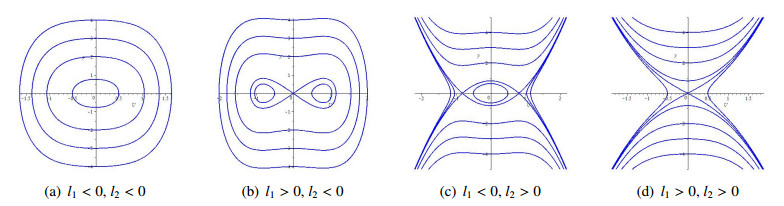
The current work studies the bifurcation and the classification of single traveling wave solutions of the coupled version of Radhakrishnan-Kundu-Lakshmanan equation that usually describes the dynamics of optical pulses in fiber Bragg gratings, which is also described by a family of nonlinear Schrödinger equations with cubic nonlinear terms. The solutions of the hyperbolic functions, the rational functions, the trigonometric functions and the Jacobian functions are retrieved by using the complete discrimination system of polynomial. By selecting appropriate parameters, phase portraits, two-dimension graphics and three-dimension graphics of the obtained solutions are drawn.
Citation: Kun Zhang, Xiaoya He, Zhao Li. Bifurcation analysis and classification of all single traveling wave solution in fiber Bragg gratings with Radhakrishnan-Kundu-Lakshmanan equation[J]. AIMS Mathematics, 2022, 7(9): 16733-16740. doi: 10.3934/math.2022918
The current work studies the bifurcation and the classification of single traveling wave solutions of the coupled version of Radhakrishnan-Kundu-Lakshmanan equation that usually describes the dynamics of optical pulses in fiber Bragg gratings, which is also described by a family of nonlinear Schrödinger equations with cubic nonlinear terms. The solutions of the hyperbolic functions, the rational functions, the trigonometric functions and the Jacobian functions are retrieved by using the complete discrimination system of polynomial. By selecting appropriate parameters, phase portraits, two-dimension graphics and three-dimension graphics of the obtained solutions are drawn.

| [1] |
A. Biswas, Optical soliton perturbation with Radhakrishnan-Kundu-Lakshmanan equation by traveling wave hypothesis, Optik, 171 (2018), 217–220. http://dx.doi.org/10.1016/j.ijleo.2018.06.043 doi: 10.1016/j.ijleo.2018.06.043

|
| [2] |
M. Annamalai, N. Veerakumar, S. Narasimhan, A. Selvaraj, Q. Zhou, A. Biswas, et al., Algorithm for dark solitons with Radhakrishnan-Kundu-Lakshmanan model in an optical fiber, Results Phys., 30 (2021), 104806. http://dx.doi.org/10.1016/j.rinp.2021.104806 doi: 10.1016/j.rinp.2021.104806
|
| [3] |
A. Biswas, M. Ekici, A. Sonmezoglu, A. Alshomrani, Optical solitons with Radhakrishnan-Kundu-Lakshmanan equation by extended trial function scheme, Optik, 160 (2018), 415–427. http://dx.doi.org/10.1016/j.ijleo.2018.02.017 doi: 10.1016/j.ijleo.2018.02.017
|
| [4] |
S. ur Rehman, J. Ahmad, Modulation instability analysis and optical solitons in birefringent fibers to RKL equation without four wave mixing, Alex. Eng. J., 60 (2021), 1339–1354. http://dx.doi.org/10.1016/j.aej.2020.10.055 doi: 10.1016/j.aej.2020.10.055
|
| [5] |
A. Biswas, Y. Yıldırım, E. Yasar, M. Mahmood, A. Alshorani, Q. Zhou, et al., Optical soliton perturbation for Radhakrishnan-Kundu-Lakshmanan equation with a couple of integration schemes, Optik, 163 (2018), 126–136. http://dx.doi.org/10.1016/j.ijleo.2018.02.109 doi: 10.1016/j.ijleo.2018.02.109
|
| [6] |
Y. Yıldırım, A. Biswas, Q. Zhou, A. Alzahrani, M. Belic, Optical solitons in birefringent fibers with Radhakrishnan-Kundu-Lakshmanan equation by a couple of strategically sound integration architectures, Chinese J. Phys., 65 (2020), 341–354. http://dx.doi.org/10.1016/j.cjph.2020.02.029 doi: 10.1016/j.cjph.2020.02.029
|
| [7] |
D. Lu, A. Seadawy, M. Khater, Dispersive optical soliton of the generalized Radhakrishnan-Kundu-Lakshmanan dynamical equation with power law nonlinearity and its applications, Optik, 164 (2018), 54–64. http://dx.doi.org/10.1016/j.ijleo.2018.02.082 doi: 10.1016/j.ijleo.2018.02.082
|
| [8] |
N. Raza, A. Javid, Dynamics of optical solitons with Radhakrishnan-Kundu-Lakshmanan model via two reliable integration schemes, Optik, 178 (2019), 557–566. http://dx.doi.org/10.1016/j.ijleo.2018.09.133 doi: 10.1016/j.ijleo.2018.09.133
|
| [9] |
A. Ghose-Choudhury, S. Garai, Solutions of the variabel coefficient Radhakrishnan-Kundu-Lakshmanan equation using the method of similarity reduction, Optik, 241 (2021), 167254. http://dx.doi.org/10.1016/j.ijleo.2021.167254 doi: 10.1016/j.ijleo.2021.167254
|
| [10] |
S. Garai, A. Ghose-Choudhury, On the solution of the generalized Radhakrishnan-Kundu-Lakshmanan equation, Optik, 243 (2021), 167374. http://dx.doi.org/10.1016/j.ijleo.2021.167374 doi: 10.1016/j.ijleo.2021.167374
|
| [11] |
G. Akram, M. Sadaf, M. Dawood, Abundant soliton solutions for Radhakrishnan-Kundu-Lakshmanan equation with Kerr law non-linearity by improved $\tan(\frac{\Phi(\xi)}{2})$-expansion technique, Optik, 247 (2021), 167787. http://dx.doi.org/10.1016/j.ijleo.2021.167787 doi: 10.1016/j.ijleo.2021.167787
|
| [12] |
W. Rabie, A. Seadawy, H. Ahmed, Highly dispersive optical solitons to the generalized third-order nonlinear Schrödinger dynamical equation with applications, Optik, 241 (2021), 167109. http://dx.doi.org/10.1016/j.ijleo.2021.167109 doi: 10.1016/j.ijleo.2021.167109
|
| [13] |
M. El-Sheikh, H. Ahmed, A. Arnous, W. Rabie, A. Biswas, A. Alshomrani, et al., Optical solitons in birefringent fibers with Lakshmanan-Porsezian-Daniel model by modified simple equation, Optik, 192 (2019), 162899. http://dx.doi.org/10.1016/j.ijleo.2019.05.105 doi: 10.1016/j.ijleo.2019.05.105
|
| [14] |
H. Eldidamony, H. Ahmed, A. Zaghrout, Y. Ali, A. Arnous, Optical solitons with Kudryashov's quintuple power law nonlinearity having nonlinear chromatic dispersion using modified extended direct algebraic method, Optik, 262 (2022), 169235. http://dx.doi.org/10.1016/j.ijleo.2022.169235 doi: 10.1016/j.ijleo.2022.169235
|
| [15] |
I. Samir, N. Badra, A. Seadawy, H. Ahmed, A. Arnous, Exact wave solutions of the fourth order nonlienar partial differential equation of optical fiber pulses by using different methods, Optik, 230 (2021), 166313. http://dx.doi.org/10.1016/j.ijleo.2021.166313 doi: 10.1016/j.ijleo.2021.166313
|
| [16] |
A. Seadawy, H. Ahmed, W. Rabie, A. Biswas, Chirp-free optical solitons in fiber bragg gratings with dispersive reflectivity having polynomial law of nonlinearity, Optik, 225 (2021), 165681. http://dx.doi.org/10.1016/j.ijleo.2020.165681 doi: 10.1016/j.ijleo.2020.165681
|
| [17] |
K. Nisar, M. Inc, A. Jhangeer, M. Muddasar, B. Infal, New soliton solutions of Heisenberg ferromagnetic spin chain model, Pramana-J. Phys., 96 (2022), 28. http://dx.doi.org/10.1007/s12043-021-02266-y doi: 10.1007/s12043-021-02266-y
|
| [18] |
M. Khater, A. Jhangeer, H. Rezazadeh, L. Akinyemi, M. Akbar, M. Inc, Propagation of new dynamics of longitudinal bud equation among a magneto-electro-elastic round rod, Mod. Phys. Lett. B, 35 (2021), 2150381. http://dx.doi.org/10.1142/S0217984921503814 doi: 10.1142/S0217984921503814
|
| [19] |
Z. Li, Bifurcation and traveling wave solution to fractional Biswas-Arshed equation with the beta time derivative, Chaos Soliton. Fract., 160 (2022), 112249. http://dx.doi.org/10.1016/j.chaos.2022.112249 doi: 10.1016/j.chaos.2022.112249
|
| [20] |
A. Jhangeer, M. Muddassar, J. Awrejcewicz, Z. Naz, M. Riaz, Phase portrait, multi-stability, sensitivity and chaotic analysis of Gardner's equation with their wave turbulence and solitons solutions, Results Phys., 32 (2022), 104981. http://dx.doi.org/10.1016/j.rinp.2021.104981 doi: 10.1016/j.rinp.2021.104981
|
| [21] |
Z. Li, Z. Lian, Optical solitons and single traveling wave solutions for the Triki-Biswas equation describing monomode optical fibers, Optik, 258 (2022), 168835. http://dx.doi.org/10.1016/j.ijleo.2022.168835 doi: 10.1016/j.ijleo.2022.168835
|
| [22] |
T. Han, Z. Li, Classification of all single traveling wave solutions of fractional coupled Boussinesq equations via the complete discrimination system method, Adv. Math. Phys., 2021 (2021), 3668063. http://dx.doi.org/10.1155/2021/3668063 doi: 10.1155/2021/3668063
|
| [23] |
T. Han, Z. Li, X. Zhang, Bifurcation and new exact traveling wave solutions to time-space coupled fractional nonlinear Schrödinger equation, Phys. Lett. A, 395 (2021), 127217. http://dx.doi.org/10.1016/j.physleta.2021.127217 doi: 10.1016/j.physleta.2021.127217
|
| [24] |
E. Zayed, R. Shohib, M. Alngar, Y. Yıldırım, Optical solitons in fiber Bragg gratings with Radhakrishnan-Kundu-Lakshmanan equation using two integration schemes, Optik, 245 (2021), 167635. http://dx.doi.org/10.1016/j.ijleo.2021.167635 doi: 10.1016/j.ijleo.2021.167635
|


Figures(3)

Kun Zhang, Xiaoya He, Zhao Li. Bifurcation analysis and classification of all single traveling wave solution in fiber Bragg gratings with Radhakrishnan-Kundu-Lakshmanan equation[J]. AIMS Mathematics, 2022, 7(9): 16733-16740. doi: 10.3934/math.2022918


 DownLoad: