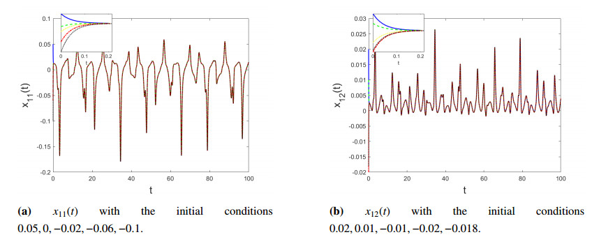
In the present paper, we prove the existence of unique almost periodic solutions to fuzzy shunting inhibitory cellular neural networks (FSICNN) with several delays. Further, by means of Halanay inequality we analyze the global exponential stability of these solutions and obtain corresponding convergence rate. The results of this paper are new, and they are concluded with numerical simulations confirming them.
Citation: Ardak Kashkynbayev, Moldir Koptileuova, Alfarabi Issakhanov, Jinde Cao. Almost periodic solutions of fuzzy shunting inhibitory CNNs with delays[J]. AIMS Mathematics, 2022, 7(7): 11813-11828. doi: 10.3934/math.2022659
In the present paper, we prove the existence of unique almost periodic solutions to fuzzy shunting inhibitory cellular neural networks (FSICNN) with several delays. Further, by means of Halanay inequality we analyze the global exponential stability of these solutions and obtain corresponding convergence rate. The results of this paper are new, and they are concluded with numerical simulations confirming them.

| [1] | A. Bouzerdoum, R. B. Pinter, Shunting inhibitory cellular neural networks: Derivation and stability analysis, IEEE T. Circuits Syst. I: Fundam. Theory Appl., 40 (1993), 215–221. |
| [2] | F. Pasemann, M. Hild, K. Zahedi, SO(2)-networks as neural oscillators, In: J. Mira, J. R. Álvarez, Computational methods in neural modeling, IWANN 2003, Lecture Notes in Computer Science, Springer, 2686 (2003), 144–151. https://doi.org/10.1007/3-540-44868-3_19 |
| [3] |
J. Cao, Global asymptotic stability of neural networks with transmission delays, Int. J. Syst. Sci., 31 (2000), 1313–1316. https://doi.org/10.1080/00207720050165807 doi: 10.1080/00207720050165807

|
| [4] |
A. Kashkynbayev, J. Cao, Z. Damiyev, Stability analysis for periodic solutions of fuzzy shunting inhibitory CNNs with delays, Adv. Differ. Equ., 2019 (2019), 384. https://doi.org/10.1186/s13662-019-2321-z doi: 10.1186/s13662-019-2321-z
|
| [5] |
J. Cao, Periodic solutions and exponential stability in delayed cellular neural networks, Phys. Rev. E, 60 (1999), 3244. https://doi.org/10.1103/PhysRevE.60.3244 doi: 10.1103/PhysRevE.60.3244
|
| [6] |
J. Cao, New results concerning exponential stability and periodic solutions of delayed cellular neural networks, Phys. Lett. A, 307 (2003), 136–147. https://doi.org/10.1016/S0375-9601(02)01720-6 doi: 10.1016/S0375-9601(02)01720-6
|
| [7] |
Z. Liu, L. Liao, Existence and global exponential stability of periodic solution of cellular neural networks with time-varying delays, J. Math. Anal. Appl., 290 (2004), 247–262. https://doi.org/10.1016/j.jmaa.2003.09.052 doi: 10.1016/j.jmaa.2003.09.052
|
| [8] |
Y. Li, Global stability and existence of periodic solutions of discrete delayed cellular neural networks, Phys. Lett. A, 333 (2004), 51–61. https://doi.org/10.1016/j.physleta.2004.10.022 doi: 10.1016/j.physleta.2004.10.022
|
| [9] |
A. Chen, J. Cao, Existence and attractivity of almost periodic solutions for cellular neural networks with distributed delays and variable coefficients, Appl. Math. Comput., 134 (2003), 125–140. https://doi.org/10.1016/S0096-3003(01)00274-0 doi: 10.1016/S0096-3003(01)00274-0
|
| [10] |
H. Jiang, L. Zhang, Z. Teng, Existence and global exponential stability of almost periodic solution for cellular neural networks with variable coefficients and time-varying delays, IEEE T. Neur. Net., 16 (2005), 1340–1351. https://doi.org/10.1109/TNN.2005.857951 doi: 10.1109/TNN.2005.857951
|
| [11] |
B. Liu, L. Huang, Existence and exponential stability of almost periodic solutions for cellular neural networks with time-varying delays, Phys. Lett. A, 341 (2005), 135–144. https://doi.org/10.1016/j.physleta.2005.04.052 doi: 10.1016/j.physleta.2005.04.052
|
| [12] |
H. Zhang, J. Shao, Almost periodic solutions for cellular neural networks with time-varying delays in leakage terms, Appl. Math. Comput., 219 (2013), 11471–11482. https://doi.org/10.1016/j.amc.2013.05.046 doi: 10.1016/j.amc.2013.05.046
|
| [13] |
Y. Yang, J. Cao, Stability and periodicity in delayed cellular neural networks with impulsive effects, Nonlinear Anal.: Real World Appl., 8 (2007), 362–374. https://doi.org/10.1016/j.nonrwa.2005.11.004 doi: 10.1016/j.nonrwa.2005.11.004
|
| [14] |
L. Pan, J. Cao, Anti-periodic solution for delayed cellular neural networks with impulsive effects, Nonlinear Anal.: Real World Appl., 12 (2011), 3014–3027. https://doi.org/10.1016/j.nonrwa.2011.05.002 doi: 10.1016/j.nonrwa.2011.05.002
|
| [15] |
K. Yuan, J. Cao, J. Deng, Exponential stability and periodic solutions of fuzzy cellular neural networks with time-varying delays, Neurocomputing, 69 (2006), 1619–1627. https://doi.org/10.1016/j.neucom.2005.05.011 doi: 10.1016/j.neucom.2005.05.011
|
| [16] |
C. Xu, Q. Zhang, Y. Wu, Existence and exponential stability of periodic solution to fuzzy cellular neural networks with distributed delays, Int. J. Fuzzy Syst., 18 (2016), 41–51. https://doi.org/10.1007/s40815-015-0103-7 doi: 10.1007/s40815-015-0103-7
|
| [17] |
Z. Huang, Almost periodic solutions for fuzzy cellular neural networks with time-varying delays, Neural Comput. Applic., 28 (2017), 2313–2320. https://doi.org/10.1007/s00521-016-2194-y doi: 10.1007/s00521-016-2194-y
|
| [18] |
Z. Huang, Almost periodic solutions for fuzzy cellular neural networks with multi-proportional delays, Int. J. Mach. Learn. Cyber., 8 (2017), 1323–1331. https://doi.org/10.1007/s13042-016-0507-1 doi: 10.1007/s13042-016-0507-1
|
| [19] |
J. Liang, H. Qian, B. Liu, Pseudo almost periodic solutions for fuzzy cellular neural networks with multi-proportional delays, Neural Process. Lett., 48 (2018), 1201–1212. https://doi.org/10.1007/s11063-017-9774-4 doi: 10.1007/s11063-017-9774-4
|
| [20] |
Y. Tang, Exponential stability of pseudo almost periodic solutions for fuzzy cellular neural networks with time-varying delays, Neural Process. Lett., 49 (2019), 851–861. https://doi.org/10.1007/s11063-018-9857-x doi: 10.1007/s11063-018-9857-x
|
| [21] |
C. Xu, M. Liao, P. Li, Z. Liu, S. Yuan, New results on pseudo almost periodic solutions of quaternion-valued fuzzy cellular neural networks with delays, Fuzzy Sets Syst., 411 (2021), 25–47. https://doi.org/10.1016/j.fss.2020.03.016 doi: 10.1016/j.fss.2020.03.016
|
| [22] |
A. Chen, J. Cao, Almost periodic solution of shunting inhibitory CNNs with delays, Phys. Lett. A, 298 (2002), 161–170. https://doi.org/10.1016/S0375-9601(02)00469-3 doi: 10.1016/S0375-9601(02)00469-3
|
| [23] |
X. Huang, J. Cao, Almost periodic solution of shunting inhibitory cellular neural networks with time-varying delay, Phys. Lett. A, 314 (2003), 222–231. https://doi.org/10.1016/S0375-9601(03)00918-6 doi: 10.1016/S0375-9601(03)00918-6
|
| [24] |
B. Liu, L. Huang, Existence and stability of almost periodic solutions for shunting inhibitory cellular neural networks with continuously distributed delays, Phys. Lett. A, 349 (2006), 177–186. https://doi.org/10.1016/j.physleta.2005.09.023 doi: 10.1016/j.physleta.2005.09.023
|
| [25] |
B. Liu, L. Huang, Existence and stability of almost periodic solutions for shunting inhibitory cellular neural networks with time-varying delays, Chaos Solitons Fract., 31 (2007), 211–217. https://doi.org/10.1016/j.chaos.2005.09.052 doi: 10.1016/j.chaos.2005.09.052
|
| [26] |
Y. Xia, J. Cao, Z. Huang, Existence and exponential stability of almost periodic solution for shunting inhibitory cellular neural networks with impulses, Chaos Solitons Fract., 34 (2007), 1599–607. https://doi.org/10.1016/j.chaos.2006.05.003 doi: 10.1016/j.chaos.2006.05.003
|
| [27] |
C. Ou, Almost periodic solutions for shunting inhibitory cellular neural networks, Nonlinear Anal.: Real World Appl., 10 (2009), 2652–2658. https://doi.org/10.1016/j.nonrwa.2008.07.004 doi: 10.1016/j.nonrwa.2008.07.004
|
| [28] |
Y. Li, C. Wang, Almost periodic solutions of shunting inhibitory cellular neural networks on time scales, Commun. Nonlinear Sci. Numer. Simul., 17 (2012), 3258–3266. https://doi.org/10.1016/j.cnsns.2011.11.034 doi: 10.1016/j.cnsns.2011.11.034
|
| [29] |
J. Shao, Anti-periodic solutions for shunting inhibitory cellular neural networks with time-varying delays, Phys. Lett. A, 372 (2008), 5011–5016. https://doi.org/10.1016/j.physleta.2008.05.064 doi: 10.1016/j.physleta.2008.05.064
|
| [30] |
G. Peng, L. Huang, Anti-periodic solutions for shunting inhibitory cellular neural networks with continuously distributed delays, Nonlinear Anal.: Real World Appl., 10 (2009), 2434–2440. https://doi.org/10.1016/j.nonrwa.2008.05.001 doi: 10.1016/j.nonrwa.2008.05.001
|
| [31] |
Y. Li, J. Shu, Anti-periodic solutions to impulsive shunting inhibitory cellular neural networks with distributed delays on time scales, Commun. Nonlinear Sci. Numer. Simul., 16 (2011), 3326–3336. https://doi.org/10.1016/j.cnsns.2010.11.004 doi: 10.1016/j.cnsns.2010.11.004
|
| [32] |
L. Peng, W. Wang, Anti-periodic solutions for shunting inhibitory cellular neural networks with time-varying delays in leakage terms, Neurocomputing, 111 (2013), 27–33. https://doi.org/10.1016/j.neucom.2012.11.031 doi: 10.1016/j.neucom.2012.11.031
|
| [33] |
Z. Long, New results on anti-periodic solutions for SICNNs with oscillating coefficients in leakage terms, Neurocomputing, 171 (2016), 503–509. https://doi.org/10.1016/j.neucom.2015.06.070 doi: 10.1016/j.neucom.2015.06.070
|
| [34] |
C. Huang, S. Wen, L. Huang, Dynamics of anti-periodic solutions on shunting inhibitory cellular neural networks with multi-proportional delays, Neurocomputing, 357 (2019), 47–52. https://doi.org/10.1016/j.neucom.2019.05.022 doi: 10.1016/j.neucom.2019.05.022
|
| [35] | T. Diagana, Almost automorphic type and almost periodic type functions in abstract spaces, New York: Springer-Verlag, 2013. https://doi.org/10.1007/978-3-319-00849-3 |
| [36] | S. Zaidman, Almost-periodic functions in abstract spaces, Pitman Research Notes in Math, Vol. 126, Boston: Pitman, 1985. |
| [37] | M. Akhmet, Almost periodicity, chaos, and asymptotic equivalence, Springer, Cham, 2020. https://doi.org/10.1007/978-3-030-20572-0 |
| [38] |
X. Huang, J. Cao, Almost periodic solution of shunting inhibitory cellular neural networks with time-varying delay, Phys. Lett. A, 314 (2003), 222–231. https://doi.org/10.1016/S0375-9601(03)00918-6 doi: 10.1016/S0375-9601(03)00918-6
|


Figures(4)

Ardak Kashkynbayev, Moldir Koptileuova, Alfarabi Issakhanov, Jinde Cao. Almost periodic solutions of fuzzy shunting inhibitory CNNs with delays[J]. AIMS Mathematics, 2022, 7(7): 11813-11828. doi: 10.3934/math.2022659


 DownLoad: