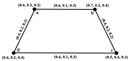
Pythagorean neutrosophic set is an extension of a neutrosophic set which represents incomplete, uncertain and imprecise details. Pythagorean neutrosophic graphs (PNG) are more flexible than fuzzy, intuitionistic, and neutrosophic models. PNG are similar in structure to fuzzy graphs but the fuzziness is more resilient when compared with other fuzzy models. In this article, regular Pythagorean neutrosophic graphs are studied, where for each element the membership $ (\mathfrak{M}) $, and non-membership $ (\mathfrak{NM}) $ are dependent and indeterminacy $ (\mathfrak{I}) $ is independently assigned. The new ideas of regular, full edge regular, edge regular, and partially edge regular Pythagorean Neutrosophic graphs are introduced and their properties are investigated. A new MCDM method has been introduced using the Pythagorean neutrosophic graphs and an illustrative example is given by applying the proposed MCDM method.
Citation: D. Ajay, P. Chellamani, G. Rajchakit, N. Boonsatit, P. Hammachukiattikul. Regularity of Pythagorean neutrosophic graphs with an illustration in MCDM[J]. AIMS Mathematics, 2022, 7(5): 9424-9442. doi: 10.3934/math.2022523
Pythagorean neutrosophic set is an extension of a neutrosophic set which represents incomplete, uncertain and imprecise details. Pythagorean neutrosophic graphs (PNG) are more flexible than fuzzy, intuitionistic, and neutrosophic models. PNG are similar in structure to fuzzy graphs but the fuzziness is more resilient when compared with other fuzzy models. In this article, regular Pythagorean neutrosophic graphs are studied, where for each element the membership $ (\mathfrak{M}) $, and non-membership $ (\mathfrak{NM}) $ are dependent and indeterminacy $ (\mathfrak{I}) $ is independently assigned. The new ideas of regular, full edge regular, edge regular, and partially edge regular Pythagorean Neutrosophic graphs are introduced and their properties are investigated. A new MCDM method has been introduced using the Pythagorean neutrosophic graphs and an illustrative example is given by applying the proposed MCDM method.

| [1] |
K. T. Atanassov, Intuitionistic fuzzy sets, Fuzzy Set. Syst., 20 (1986), 87–96. https://doi.org/10.1016/S0165-0114(86)80034-3 doi: 10.1016/S0165-0114(86)80034-3

|
| [2] |
L. A. Zadeh, Fuzzy sets, Information and Control, 8 (1965), 338–353. https://doi.org/10.2307/2272014 doi: 10.2307/2272014
|
| [3] |
X. He, Y. Wu, D. Yu, Intuitionistic fuzzy multi-criteria decision making with application to job hunting: A comparative perspective, J. Intell. Fuzzy Syst., 30 (2016), 1935–1946. https://doi.org/10.3233/IFS-151904 doi: 10.3233/IFS-151904
|
| [4] |
S. Zeng, Y. Xiao, TOPSIS method for intuitionistic fuzzy multiple-criteria decision making and its application to investment selection, Kybernetes, 45 (2016), 282–296. https://doi.org/10.1108/K-04-2015-0093 doi: 10.1108/K-04-2015-0093
|
| [5] |
Z. Wang, Z. Xu, S. Liu, J. Tang, A netting clustering analysis method under intuitionistic fuzzy environment, Appl. Soft Comput., 11 (2011), 5558–5564. https://doi.org/10.1016/j.asoc.2011.05.004 doi: 10.1016/j.asoc.2011.05.004
|
| [6] |
K. I. Vlachos, G. D. Sergiadis, Intuitionistic fuzzy information-applications to pattern recognition, Pattern Recogn. Lett., 28 (2007), 197–206. https://doi.org/10.1016/j.patrec.2006.07.004 doi: 10.1016/j.patrec.2006.07.004
|
| [7] |
Z. Z. Liang, P. F. Shi, Similarity measures on intuitionistic fuzzy sets, Pattern Recogn. Lett., 24 (2003), 2687–2693. https://doi.org/10.1016/S0167-8655(03)00111-9 doi: 10.1016/S0167-8655(03)00111-9
|
| [8] |
S. K. De, R. Biswas, A. R. Roy, An application of intuitionistic fuzzy sets in medical diagnosis, Fuzzy Set. Syst., 117 (2001), 209–213. https://doi.org/10.1016/S0165-0114(98)00235-8 doi: 10.1016/S0165-0114(98)00235-8
|
| [9] | F. Smarandache, A unifying field in logics. Neutrosophy: neutrosophic probability, set and logic, Rehoboth: American Research Press, 1999. |
| [10] | H. Wang, F. Smarandache, Y. Q. Zhang, R. Sunderraman, Single valued neutrosophic sets, 2010. |
| [11] |
Y. Guo, H. D. Cheng, New neutrosophic approach to image segmentation, Pattern Recogn., 42 (2009), 587–595. https://doi.org/10.1016/j.patcog.2008.10.002 doi: 10.1016/j.patcog.2008.10.002
|
| [12] |
J. Ye, J. Fu, Multi-period medical diagnosis method using a single valued neutrosophic similarity measure based on tangent function, Comput. Meth. Prog. Bio., 123 (2016), 142–149. https://doi.org/10.1016/j.cmpb.2015.10.002 doi: 10.1016/j.cmpb.2015.10.002
|
| [13] |
J. Ye, Multicriteria decision-making method using the correlation coefficient under single valued neutrosophic environment, Int. J. Gen. Syst., 42 (2013), 386–394. https://doi.org/10.1080/03081079.2012.761609 doi: 10.1080/03081079.2012.761609
|
| [14] | S. Bhattacharya, Neutrosophic information fusion applied to the options market, Investment Management and Financial Innovations, 1 (2005), 139–145. |
| [15] | S. Aggarwal, R. Biswas, A. Q. Ansari, Neutrosophic modeling and control, 2010 International Conference on Computer and Communication Technology (ICCCT), 2010,718–723. https://doi.org/10.1109/ICCCT.2010.5640435 |
| [16] | S. Y. Wu, Y. M. Kao, The compositions of fuzzy digraphs, J. Res. Educ. Sci., 31 (1986), 603–628. |
| [17] |
H. L. Yang, Z. L. Guo, Y. She, X. Liao, On single valued neutrosophic relations, J. Intell. Fuzzy Syst., 30 (2016), 1045–1056. https://doi.org/10.3233/IFS-151827 doi: 10.3233/IFS-151827
|
| [18] | R. R. Yager, Pythagorean fuzzy subsets, In: Proceedings of the Joint IFSA World Congress and NAFIPS Annual Meeting, Edmonton, AB, Canada, 2013, 57–61. https://doi.org/10.1109/IFSA-NAFIPS.2013.6608375 |
| [19] |
R. R. Yager, A. M. Abbasov, Pythagorean membership grades, complex numbers and decision making, Int. J. Intell. Syst., 28 (2013), 436–452. https://doi.org/10.1002/int.21584 doi: 10.1002/int.21584
|
| [20] |
R. R. Yager, Pythagorean membership grades in multi-criteria decision making, IEEE Trans. Fuzzy Syst., 22 (2014), 958–965. https://doi.org/10.1109/TFUZZ.2013.2278989 doi: 10.1109/TFUZZ.2013.2278989
|
| [21] | R. Jansi, K. Mohana, F. Smarandache, Correlation measure for pythagorean neutrosophic sets with t and f as dependent neutrosophic components, Neutrosophic Sets and Systems, 30 (2019), 202–212. |
| [22] | A. Kauffman, Introduction a la Theorie des Sous-emsembles Flous, Masson et Cie., 1 (1973). |
| [23] | A. Rosenfeld, Fuzzy graphs, In: Fuzzy sets and their applications to cognitive and decision processes, New York: Academic Press, 1975, 77–95. https://doi.org/10.1016/B978-0-12-775260-0.50008-6 |
| [24] |
P. Bhattacharya, Some remarks on fuzzy graphs, Pattern Recogn. Lett., 6 (1987), 297–302. https://doi.org/10.1016/0167-8655(87)90012-2 doi: 10.1016/0167-8655(87)90012-2
|
| [25] | K. Radha, N. Kumaravel, On edge regular fuzzy graphs, International Journal of Mathematical Archive, 5 (2014), 100–112. |
| [26] | K. T. Atanassov, Intuitionistic fuzzy sets, In: Intuitionistic fuzzy sets, Heidelberg: Physica, 1999, 1–137. https://doi.org/10.1007/978-3-7908-1870-3_1 |
| [27] |
M. Akram, B. Davvaz, Strong intuitionistic fuzzy graphs, Filomat, 26 (2012), 177–196. https://doi.org/10.2298/FIL1201177A doi: 10.2298/FIL1201177A
|
| [28] | M. G. Karunambigai, S. Sivasankar, K. Palanivel, Some properties of a regular intuitionistic fuzzy graph, International Journal of Mathematics and Computation, 26 (2015), 53–61. |
| [29] |
M. G. Karunambigai, K. Palanivel, S. Sivasankar, Edge regular intuitionistic fuzzy graph, Advances in Fuzzy Sets and Systems, 20 (2015), 25–46. http://dx.doi.org/10.17654/AFSSSep2015_025_046 doi: 10.17654/AFSSSep2015_025_046
|
| [30] |
R. A. Borzooei, H. Rashmanlou, S. Samanta, M. Pal, Regularity of vague graphs, J. Intell. Fuzzy Syst., 30 (2016), 3681–3689. https://doi.org/10.3233/IFS-162114 doi: 10.3233/IFS-162114
|
| [31] | S. N. Mishra, A. Pal, Product of interval-valued intuitionistic fuzzy graph, Annals of Pure and Applied Mathematics, 5 (2013), 37–46. |
| [32] | W. B. Vasantha Kandasamy, K. Ilanthenral, F. Smarandache, Neutrosophic graphs: A new dimension to graph theory, 2015. |
| [33] | S. Broumi, M. Talea, A. Bakali, F. Smarandache, On bipolar single valued neutrosophic graphs, Journal of New Theory, 2016 (2016), 84–102. |
| [34] | S. Broumi, M. Talea, A. Bakali, F. Smarandache, Interval valued neutrosophic graphs, Critical Review, XII (2016), 5–33. |
| [35] |
S. Naz, S. Ashraf, M. Akram, A novel approach to decision making with Pythagorean fuzzy information, Mathematics, 6 (2018), 95. https://doi.org/10.3390/math6060095 doi: 10.3390/math6060095
|
| [36] | D. Ajay, P. Chellamani, Pythagorean neutrosophic fuzzy graphs, International Journal of Neutrosophic Science, 11 (2020), 108–114. |
| [37] | M. Doumpos, C. Zopounidis, Multicriteria decision aid classification methods, Boston, MA: Springer, 2002. https://doi.org/10.1007/b101986 |
| [38] |
P. Agarwal, M. Ramadan, H. S. Osheba, Y. M. Chu, Study of hybrid orthonormal functions method for solving second kind fuzzy Fredholm integral equations, Adv. Differ. Equ., 2020 (2020), 533. https://doi.org/10.1186/s13662-020-02985-3 doi: 10.1186/s13662-020-02985-3
|
| [39] |
S. Singh, A. H. Ganie, Applications of picture fuzzy similarity measures in pattern recognition, clustering, and MADM, Expert Syst. Appl., 168 (2021), 114–264. https://doi.org/10.1016/j.eswa.2020.114264 doi: 10.1016/j.eswa.2020.114264
|
| [40] |
K. R. Mokarrari, S. A. Torabi, Ranking cities based on their smartness level using MADM methods, Sustain. Cities Soc., 72 (2021), 103030. https://doi.org/10.1016/j.scs.2021.103030 doi: 10.1016/j.scs.2021.103030
|
| [41] |
H. A. Hammad, M. De la Sen, P. Agarwal, New coincidence point results for generalized graph-preserving multivalued mappings with applications, Adv. Differ. Equ., 2021 (2021), 334. https://doi.org/10.1186/s13662-021-03489-4 doi: 10.1186/s13662-021-03489-4
|
| [42] | O. Grigorenko, Fuzzy metrics for solving MODM problems, In: 19th World Congress of the International Fuzzy Systems Association (IFSA), 12th Conference of the European Society for Fuzzy Logic and Technology (EUSFLAT), and 11th International Summer School on Aggregation Operators (AGOP), Atlantis Press, 2021,360–366. https://doi.org/10.2991/asum.k.210827.048 |
| [43] |
W. B. Jurkat, H. J. Ryser, Matrix factorizations of determinants and permanents, J. Algebra, 3 (1966), 1–27. https://doi.org/10.1016/0021-8693(66)90016-0 doi: 10.1016/0021-8693(66)90016-0
|
| [44] | T. Rasham, M. S. Shabbir, P. Agarwal, S. Momani, On a pair of fuzzy dominated mappings on closed ball in the multiplicative metric space with applications, Fuzzy Set. Syst., in press. https://doi.org/10.1016/j.fss.2021.09.002 |
| [45] | A. Singh, P. Agarwal, M. Chand, Image encryption and analysis using dynamic AES, In: 2019 5th International Conference on Optimization and Applications (ICOA), IEEE, 2019, 1–6. https://doi.org/10.1109/ICOA.2019.8727711 |
| [46] | S. J. Chen, C. L. Hwang, Fuzzy multiple attribute decision making methods, In: Fuzzy multiple attribute decision making, Berlin, Heidelberg: Springer, 1992,289–486. https://doi.org/10.1007/978-3-642-46768-4_5 |
| [47] |
P. Agarwal, M. Chand, J. Choi, G. Singh, Certain fractional integrals and image formulas of generalized k-Bessel function, Commun. Korean Math. Soc., 33 (2018), 423–436. https://doi.org/10.4134/CKMS.c170056 doi: 10.4134/CKMS.c170056
|
| [48] | G. Rajchakit, P. Agarwal, S. Ramalingam, Stability analysis of neural networks, Singapore: Springer, 2021. https://doi.org/10.1007/978-981-16-6534-9 |
| [49] |
C. Carlsson, R. Fuller, Fuzzy multiple criteria decision making: recent developments, Fuzzy Set. Syst., 78 (1996), 139–153. https://doi.org/10.1016/0165-0114(95)00165-4 doi: 10.1016/0165-0114(95)00165-4
|
| [50] |
R. V. Rao, A decision-making framework model for evaluating flexible manufacturing systems using digraph and matrix methods, Int. J. Adv. Manuf. Technol., 30 (2006), 1101–1110. https://doi.org/10.1007/s00170-005-0150-6 doi: 10.1007/s00170-005-0150-6
|
| [51] |
R. A. Ribeiro, Fuzzy multiple attribute decision making: a review and new preference elicitation techniques, Fuzzy Set. Syst., 78 (1996), 155–181. https://doi.org/10.1016/0165-0114(95)00166-2 doi: 10.1016/0165-0114(95)00166-2
|
| [52] |
E. Triantaphyllou, C. T. Lin, Development and evaluation of five fuzzy multiattribute decision-making methods, Int. J. Approx. Reason., 14 (1996), 281–310. https://doi.org/10.1016/0888-613X(95)00119-2 doi: 10.1016/0888-613X(95)00119-2
|
| [53] | P. Chellamani, D. Ajay, Pythagorean neutrosophic Dombi fuzzy graphs with an application to MCDM, Neutrosophic Sets and Systems, 47 (2021), 411–431. |
| [54] | P. Chellamani, D. Ajay, S. Broumi, T. Ligori, An approach to decision-making via picture fuzzy soft graphs, Granul. Comput., 2021, in press. https://doi.org/10.1007/s41066-021-00282-2 |
| [55] |
L. Abdullah, Fuzzy multi criteria decision making and its applications: A brief review of category, Procedia-Social and Behavioral Sciences, 97 (2013), 131–136. https://doi.org/10.1016/j.sbspro.2013.10.213 doi: 10.1016/j.sbspro.2013.10.213
|
| [56] | D. Ajay, P. Chellamani, Pythagorean neutrosophic soft sets and their application to decision-making scenario, In: Intelligent and Fuzzy Techniques for Emerging Conditions and Digital Transformation. INFUS 2021, Cham: Springer, 2021,552–560. https://doi.org/10.1007/978-3-030-85577-2_65 |
| [57] | S. Broumi, M. Talea, A. Bakali, F. Smarandache, Single valued neutrosophic graphs, Journal of New Theory, 2016 (2016), 86–101. |
| [58] |
R. Sahin, An approach to neutrosophic graph theory with applications, Soft Comput., 23 (2019), 569–581. https://doi.org/10.1007/s00500-017-2875-1 doi: 10.1007/s00500-017-2875-1
|


Figures(3) / Tables(1)

D. Ajay, P. Chellamani, G. Rajchakit, N. Boonsatit, P. Hammachukiattikul. Regularity of Pythagorean neutrosophic graphs with an illustration in MCDM[J]. AIMS Mathematics, 2022, 7(5): 9424-9442. doi: 10.3934/math.2022523


 DownLoad: