Aiming at the problem of solving nonlinear ordinary differential equations with variable coefficients, this paper introduces the elastic transformation method into the process of solving ordinary differential equations for the first time. A class of first-order and a class of third-order ordinary differential equations with variable coefficients can be transformed into the Laguerre equation through elastic transformation. With the help of the general solution of the Laguerre equation, the general solution of these two classes of ordinary differential equations can be obtained, and then the curves of the general solution can be drawn. This method not only expands the solvable classes of ordinary differential equations, but also provides a new idea for solving ordinary differential equations with variable coefficients.
Citation: Pengshe Zheng, Jing Luo, Shunchu Li, Xiaoxu Dong. Elastic transformation method for solving ordinary differential equations with variable coefficients[J]. AIMS Mathematics, 2022, 7(1): 1307-1320. doi: 10.3934/math.2022077
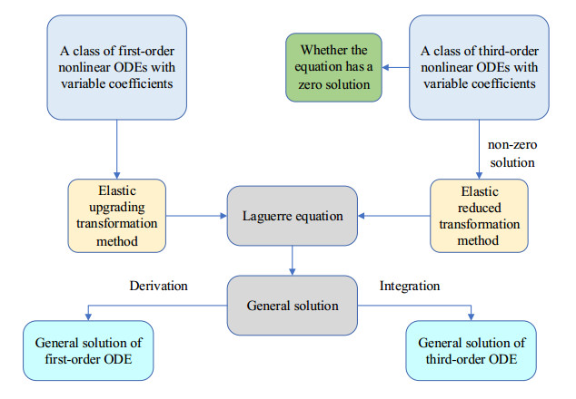
Aiming at the problem of solving nonlinear ordinary differential equations with variable coefficients, this paper introduces the elastic transformation method into the process of solving ordinary differential equations for the first time. A class of first-order and a class of third-order ordinary differential equations with variable coefficients can be transformed into the Laguerre equation through elastic transformation. With the help of the general solution of the Laguerre equation, the general solution of these two classes of ordinary differential equations can be obtained, and then the curves of the general solution can be drawn. This method not only expands the solvable classes of ordinary differential equations, but also provides a new idea for solving ordinary differential equations with variable coefficients.

| [1] | M. Alfred, Principles of Economics, London Macmillan and Co., 1920,102–116. |
| [2] | E. Bicer, On the asymptotic behavior of solutions of neutral mixed type differential equations, Results Math., 144 (2018). doi: 10.1007/s00025-018-0906-6. |
| [3] |
S. S. Fang, The operator solution of third-order variable coefficient linear differential equations, Editorial Dep. Shantou Univ. J., 26 (2011), 3–9. doi:10.3969/j.issn.1001-4217.2011.03.002. doi: 10.3969/j.issn.1001-4217.2011.03.002

|
| [4] |
D. D. Gui, S. C. Li, L. Ren, A method for solving a class of boundary value problems of Laguerre equation, Am. J. Appl. Math. Stat., 3 (2015), 89–92. doi: 10.12691/ajams-3-3-1. doi: 10.12691/ajams-3-3-1
|
| [5] |
Q. M. Gui, S. C. Li, C. C. Zhao, P. S. Zheng, Analysis of oil and gas flow characteristics in the reservoir with the elastic outer boundary, J. Petrol. Sci. Eng., 175 (2019), 280–85. doi: 10.1016/j.petrol.2018.12.042. doi: 10.1016/j.petrol.2018.12.042
|
| [6] |
H. Guo, S. C. Li, P. S. Zheng, The elastic boundary value problem of extended modified Bessel equation and its application in fractal homogeneous reservoir, Comput. Appl. Math., 39 (2020), 63. doi: 10.1007/s40314-020-1104-1. doi: 10.1007/s40314-020-1104-1
|
| [7] |
W. Guo, Solving a kind of third-order linear differential equations with variable coefficients and its realization in Maple, J. Xinzhou Teachers Univ., 32 (2012), 5–7. doi: 10.3969/j.issn.1671-1491.2016.02.002. doi: 10.3969/j.issn.1671-1491.2016.02.002
|
| [8] |
A. M. Ishkhanyan, D. A. Satco, S. Y. Slavyanov, Generation and removal of apparent singularities in linear ordinary differential equations with polynomial coefficients, Theor. Math. Phys., 189 (2016), 1726–1733. doi: 10.1134/S0040577916120059. doi: 10.1134/S0040577916120059
|
| [9] |
Y. P. Jia, L. P. Li, Three types of third-order nonlinear differential equations that can be reduced, J. Shanxi Datong Univ., 32 (2016), 1–2. doi: 10.3969/j.issn.1674-0874.2016.06.001. doi: 10.3969/j.issn.1674-0874.2016.06.001
|
| [10] |
H. John, Sauro, Herbert, M. Woods, Elasticities in metabolic control analysis: Algebraic derivation of simplified expressions, Comput. Appl. Biosci., 13 (1997), 123–130. doi: 10.1093/bioinformatics/13.2.123. doi: 10.1093/bioinformatics/13.2.123
|
| [11] |
S. Y. Li, The general solution of a class of n-th order variable coefficient linear ordinary differential equations, J. Wenshan Univ., 23 (2010), 106–109. doi: 10.3969/j.issn.1674-9200.2007.03.020. doi: 10.3969/j.issn.1674-9200.2007.03.020
|
| [12] | S. D. Liu, S. S. Liu, Special Functions, 2 Eds., Beijing: China Meteorological Press, 2002. |
| [13] |
Waleed M. Alfaqih, Abdullah Aldurayhim, Mohammad Imdad, Atiya Perveen, Relation-theoretic fixed point theorems under a new implicit function with applications to ordinary differential equations, AIMS Math., 5 (2020), 6766–6781. doi: 10.3934/math.2020435. doi: 10.3934/math.2020435
|
| [14] | K. Murase, Igaku Butsuri: Nihon Igaku Butsuri Gakkai Kikanshi = Japanese Journal of Medical Physics: An Official Journal of Japan Society of Medical Physics, 344 (2014), 227–35. |
| [15] |
M. Naito, Oscillation and nonoscillation of solutions of a second-order nonlinear ordinary differential equation, Results Math., 74 (2019), 178. doi: 10.1007/s00025-019-1103-y. doi: 10.1007/s00025-019-1103-y
|
| [16] |
K. Schmitt, J. R. Ward, Almost periodic solutions of nonlinear second order differential equations, Results Math., 21 (1992), 190–199. doi: 10.1007/BF03323078. doi: 10.1007/BF03323078
|
| [17] | G. X. Wang, Ordinary Differential Equations, 3 Eds., Beijing: Higher Education Press, 2006. |
| [18] |
J. Q. Wu, Solving a class of first-order linear differential equations with the "upgrading method"——Also on the cultivation of reverse thinking ability, Studies Coll. Math., 19 (2016), 26–28. doi: 10.3969/j.issn.1008-1399.2016.03.010. doi: 10.3969/j.issn.1008-1399.2016.03.010
|
| [19] | J. P. Zhang, The general concept of elasticity coefficient, Tech. Econ., 1995. |
| [20] | V. F. Zaitsev, A. D. Polyanin, Handbook of Exact Solutions for Ordinary Differential Equations, CRC press, 2002. |


Figures(6)

Pengshe Zheng, Jing Luo, Shunchu Li, Xiaoxu Dong. Elastic transformation method for solving ordinary differential equations with variable coefficients[J]. AIMS Mathematics, 2022, 7(1): 1307-1320. doi: 10.3934/math.2022077


 DownLoad: