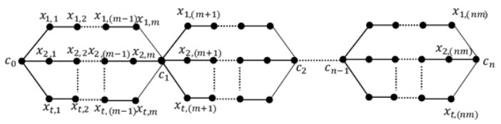
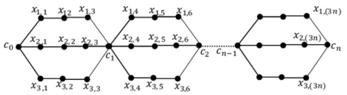
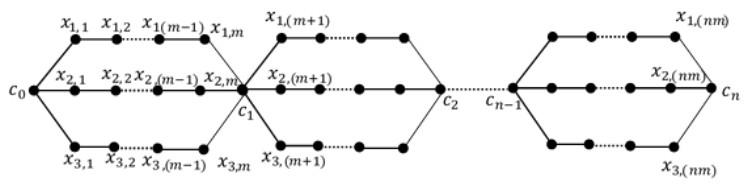
A labeling of a connected, simple and undirected graph G(V, E) is a map that assigns the elements of a graph G with positive numbers. Many types of labeling for graph are found and one of them is a total edge irregularity strength (TEIS) of G, which denoted by tes(G). In the current paper, we defined a new type of family of graph called uniform theta snake graph, $\theta_{n}(t, m)$. Also, the exact values of total edge irregularity strengths for some special types of the new family have been determined.
Citation: Fatma Salama, Randa M. Abo Elanin. On total edge irregularity strength for some special types of uniform theta snake graphs[J]. AIMS Mathematics, 2021, 6(8): 8127-8148. doi: 10.3934/math.2021471
A labeling of a connected, simple and undirected graph G(V, E) is a map that assigns the elements of a graph G with positive numbers. Many types of labeling for graph are found and one of them is a total edge irregularity strength (TEIS) of G, which denoted by tes(G). In the current paper, we defined a new type of family of graph called uniform theta snake graph, $\theta_{n}(t, m)$. Also, the exact values of total edge irregularity strengths for some special types of the new family have been determined.

| [1] | A. Ahmad, M. K. Siddiqui, D. Afzal, On the total edge irregularity strength of zigzag graphs, Australas. J. Comb., 54 (2012), 141-149. |
| [2] |
A. Ahmad, M. Arshad, G. Ižaríková, Irregular labelings of helm and sun graphs, AKCE Int. J. Graphs Combinatorics, 12 (2015), 161-168. doi: 10.1016/j.akcej.2015.11.010

|
| [3] |
A. Ahmad, M. Bača, M. K. Siddiqui, On edge irregular total labeling of categorical product of two cycles, Theory Comput. Syst., 54 (2014), 1-12. doi: 10.1007/s00224-013-9470-3
|
| [4] | A. Ahmad, M. Bača, Total edge irregularity strength of a categorical product of two paths, Ars Comb., 114 (2014), 203-212. |
| [5] | A. Ahmad, O. B. S. Al-Mushayt, M. Bača, On edge irregularity strength of graphs, Appl. Math. Comput., 243 (2014), 607-610. |
| [6] | A. Ahmad, M. K. Siddiqui, M. Ibrahim, M. Asif, On the total irregularity strength of generalized Petersen graph, Math. Rep., 18 (2016), 197-204. |
| [7] | A. Ahmad, M. Bača, Edge irregular total labeling of certain family of graphs, AKCE Int. J. Graphs. Combinatorics, 6 (2009), 21-29. |
| [8] | O. Al-Mushayt, A. Ahmad, M. K. Siddiqui, On the total edge irregularity strength of hexagonal grid graphs, Australas. J. Comb., 53 (2012), 263-271. |
| [9] |
D. Amar, O. Togni, Irregularity strength of trees, Discrete Math., 190 (1998), 15-38. doi: 10.1016/S0012-365X(98)00112-5
|
| [10] |
M. Bača, S. Jendroî, M. Miller, J. Ryan, On irregular total labellings, Discrete Math., 307 (2007), 1378-1388. doi: 10.1016/j.disc.2005.11.075
|
| [11] | M. Bača, M. K. Siddiqui, Total edge irregularity strength of generalized prism, Appl. Math. Comput., 235 (2014), 168-173. |
| [12] |
S. Brandt, J. Miškuf, D. Rautenbach, On a conjecture about edge irregular total labellings, J. Graph Theory, 57 (2008), 333-343. doi: 10.1002/jgt.20287
|
| [13] |
N. Hinding, N. Suardi, H. Basir, Total edge irregularity strength of subdivision of star, J. Discrete Math. Sci. Cryptography, 18 (2015), 869-875. doi: 10.1080/09720529.2015.1032716
|
| [14] |
D. Indriati, Widodo, I. E. Wijayanti, K. A. Sugeng, M. Bača, On total edge irregularity strength of generalized web graphs and related graphs, Math. Comput. Sci., 9 (2015), 161-167. doi: 10.1007/s11786-015-0221-5
|
| [15] |
J. Ivanĉo, S. Jendroî, Total edge irregularity strength of trees, Discussiones Math. Graph Theory, 26 (2006), 449-456. doi: 10.7151/dmgt.1337
|
| [16] |
S. Jendroî, J. Miŝkuf, R. Soták, Total edge irregularity strength of complete graph and complete bipartite graphs, Electron. Notes Discrete Math., 28 (2007), 281-285. doi: 10.1016/j.endm.2007.01.041
|
| [17] |
P. Jeyanthi, A. Sudha, Total edge irregularity strength of disjoint union of wheel graphs, Electron. Notes Discrete Math., 48 (2015), 175-182. doi: 10.1016/j.endm.2015.05.026
|
| [18] |
P. Majerski, J. Przybylo, On the irregularity strength of dense graphs, SIAM J. Discrete Math., 28 (2014), 197-205. doi: 10.1137/120886650
|
| [19] | J. Miškuf, S. Jendroî, On total edge irregularity strength of the grids, Tatra Mt. Math. Publ., 36 (2007), 147-151. |
| [20] |
M. Naeem, M. K. Siddiqui, Total irregularity strength of disjoint union of isomorphic copies of generalized Petersen graph, Discrete Math. Algorithms Appl., 9 (2017), 1750071. doi: 10.1142/S1793830917500719
|
| [21] |
F. Pfender, Total edge irregularity strength of large graphs, Discrete Math., 312 (2012), 229-237. doi: 10.1016/j.disc.2011.08.027
|
| [22] |
R. W. Putra, Y. Susanti, On total edge irregularity strength of centralized uniform theta graphs, AKCE Int. J. Graphs Combinatorics, 15 (2018), 7-13. doi: 10.1016/j.akcej.2018.02.002
|
| [23] |
B. Rajan, I. Rajasingh, P. Venugopal, Metric dimension of uniform and quasi-uniform theta graphs, J. Comput. Math. Sci., 2 (2011), 37-46. doi: 10.22436/jmcs.002.01.05
|
| [24] | I. Rajasingh, S. T. Arockiamary, Total edge irregularity strength of series parallel graphs, Int. J. Pure Appl. Math., 99 (2015), 11-21. |
| [25] | R. Ramdani, A. N. M. Salman, On the total irregularity strength of some Cartesian product graphs, AKCE Int. J. Graphs Combinatorics, 10 (2013), 199-209. |
| [26] |
F. Salama, On total edge irregularity strength of polar grid graph, J. Taibah Univ. Sci., 13 (2019), 912-916. doi: 10.1080/16583655.2019.1660086
|
| [27] | F. Salama, Exact value of total edge irregularity strength for special families of graphs, An. Univ. Oradea, Fasc. Math., 26 (2020), 123-130. |
| [28] | F. Salama, Computing the total edge irregularity strength for quintet snake graph and related graphs, J. Discrete Math. Sci. Cryptography, (2021), 1-14. Available from: https://doi.org/10.1080/09720529.2021.1878627. |
| [29] | M. K. Siddiqui, On edge irregularity strength of subdivision of star Sn, Int. J. Math. Soft Comput., 2 (2012), 75-82. |
| [30] |
I. Tarawneh, R. Hasni, A. Ahmad, M. A. Asim, On the edge irregularity strength for some classes of plane graphs, AIMS Math., 6 (2021), 2724-2731. doi: 10.3934/math.2021166
|
| [31] | M. I. Tilukay, A. N. M. Salman, E. R. Persulessy, On the total irregularity strength of fan, wheel, triangular book, and friendship graphs, Procedia Comput. Sci., 74 (2015), 124-131. |
| [32] |
H. Yang, M. K. Siddiqui, M. Ibrahim, S. Ahmad, A. Ahmad, Computing the irregularity strength of planar graphs, Mathematics, 6 (2018), 150. doi: 10.3390/math6090150
|
Figures(3)

Fatma Salama, Randa M. Abo Elanin. On total edge irregularity strength for some special types of uniform theta snake graphs[J]. AIMS Mathematics, 2021, 6(8): 8127-8148. doi: 10.3934/math.2021471


 DownLoad: