Impulsive control strategy for the Mittag-Leffler synchronization of fractional-order neural networks with mixed bounded and unbounded delays

Ivanka Stamova; Gani Stamov; Ivanka Stamova; Gani Stamov

doi:10.3934/math.2021138

AIMS Mathematics

2021, Volume 6, Issue 3: 2287-2303. doi: 10.3934/math.2021138

Previous Article Next Article

Research article Special Issues

Impulsive control strategy for the Mittag-Leffler synchronization of fractional-order neural networks with mixed bounded and unbounded delays

Ivanka Stamova ^{1
,
,},
Gani Stamov ²

1.
Department of Mathematics, University of Texas at San Antonio, San Antonio, TX 78249, USA
2.
Department of Mathematics, Technical University of Sofia, Bulgaria

Received: 09 November 2020 Accepted: 11 December 2020 Published: 15 December 2020
MSC : 26A33, 34K37, 34K45, 34K25, 34K60

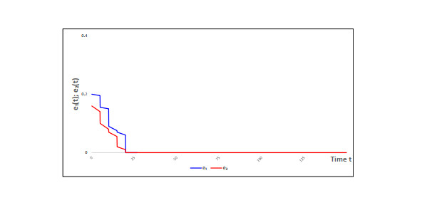
In this paper we apply an impulsive control method to keep the Mittag-Leffler stability properties for a class of Caputo fractional-order cellular neural networks with mixed bounded and unbounded delays. The impulsive controls are realized at fixed moments of time. Our results generalize some known criteria to the fractional-order case and provide a design method of impulsive control law for the impulse free fractional-order neural network model. Examples are presented to demonstrate the effectiveness of our results.
- global Mittag-Leffler synchronization,
- neural networks,
- fractional-order derivatives,
- mixed delays,
- impulsive control
Citation: Ivanka Stamova, Gani Stamov. Impulsive control strategy for the Mittag-Leffler synchronization of fractional-order neural networks with mixed bounded and unbounded delays[J]. AIMS Mathematics, 2021, 6(3): 2287-2303. doi: 10.3934/math.2021138

Related Papers:

Abstract

In this paper we apply an impulsive control method to keep the Mittag-Leffler stability properties for a class of Caputo fractional-order cellular neural networks with mixed bounded and unbounded delays. The impulsive controls are realized at fixed moments of time. Our results generalize some known criteria to the fractional-order case and provide a design method of impulsive control law for the impulse free fractional-order neural network model. Examples are presented to demonstrate the effectiveness of our results.

References

[1]	S. Abbas, M. Banerjee, S. Momani, Dynamical analysis of fractional-order modified logistic model, Comput. Math. Appl., 62 (2011), 1098-1104. doi: 10.1016/j.camwa.2011.03.072
[2]	S. Das, P. K. Gupta, A mathematical model on fractional Lotka-Volterra equations, J. Theor. Biol., 277 (2011), 1-6. doi: 10.1016/j.jtbi.2011.01.034
[3]	H. L. Li, L. Zhang, C. Hu, Y. L. Jiang, Z. Teng, Dynamical analysis of a fractional-order predator-prey model incorporating a prey refuge, J. Appl. Math. Comput., 54 (2017), 435-449. doi: 10.1007/s12190-016-1017-8
[4]	G. Stamov, I. Stamova, Modelling and almost periodic processes in impulsive Lasota-Wazewska equations of fractional order with time-varying delays, Quaest. Math., 40 (2017), 1041-1057. doi: 10.2989/16073606.2017.1346717
[5]	E. H. Dulf, D. C. Vodnar, A. Danku, C. I. Muresan, O. Crisan, Fractional‐order models for biochemical processes, Fractal Fract., 4 (2020), 12. doi: 10.3390/fractalfract4020012
[6]	B. N. Lundstrom, M. H. Higgs, W. J. Spain, A. L. Fairhall, Fractional differentiation by neocortical pyramidal neurons, Nat. Neurosci., 11 (2008), 1335-1342. doi: 10.1038/nn.2212
[7]	R. L. Magin, Fractional calculus in bioengineering, Redding: Begell House, 2006.
[8]	W. Teka, T. M. Marinov, F. Santamaria, Neuronal spike timing adaptation described with a fractional leaky integrate-and-fire model, PLoS Comput. Biol., 10 (2014), e1003526. doi: 10.1371/journal.pcbi.1003526
[9]	K. Sayevand, A study on existence and global asymptotical Mittag-Leffler stability of fractional Black-Scholes equation for a European option pricing equation, J. Hyperstruct., 3 (2014), 126-138.
[10]	J. J. Nieto, G. T. Stamov, I. M. Stamova, A fractional-order impulsive delay model of price fluctuations in commodity markets: Almost periodic solutions, Eur. Phys. J. Spec. Top., 226 (2017), 3811-3825. doi: 10.1140/epjst/e2018-00033-9
[11]	A. Atangana, Fractal-fractional differentiation and integration: Connecting fractal calculus and fractional calculus to predict complex system, Chaos Solitons Fractals, 102 (2017), 396-406. doi: 10.1016/j.chaos.2017.04.027
[12]	D. Baleanu, K. Diethelm, E. Scalas, J. J. Trujillo, Fractional calculus: Models and numerical methods, Hackensack: World Scientific, 2012.
[13]	R. Hilfer, Application of fractional calculus in physics, River Edge: World Scientific, 2000.
[14]	I. Podlubny, Fractional differential equations, San Diego: BAcademic Press, 1999.
[15]	I. M. Stamova, G. T. Stamov, Functional and impulsive differential equations of fractional order: Qualitative analysis and applications, Boca-Raton: CRC Press, 2017.
[16]	H. Bao, J. H. Park, J. Cao, Non-fragile state estimation for fractional-order delayed memristive BAM neural networks, Neural Networks, 119 (2019), 190-199. doi: 10.1016/j.neunet.2019.08.003
[17]	H. L. Li, H. Jiang, J. Cao, Global synchronization of fractional-order quaternion-valued neural networks with leakage and discrete delays, Neurocomputing, 385 (2020), 211-219. doi: 10.1016/j.neucom.2019.12.018
[18]	X. Peng, H. Wu, J. Cao, Global nonfragile synchronization in finite time for fractional-order discontinuous neural networks with nonlinear growth activations, IEEE Trans. Neural Networks Learn. Syst., 30 (2019), 2123-2137. doi: 10.1109/TNNLS.2018.2876726
[19]	R. Rakkiyappan, C. Velmurugan, J. Cao, Stability analysis of memristor-based fractional-order neural networks with different memductance functions, Cogn. Neurodynamics, 9 (2015), 145-177. doi: 10.1007/s11571-014-9312-2
[20]	I. M. Stamova, S. Simeonov, Delayed reaction-diffusion cellular neural networks of fractional order: Mittag-Leffler stability and synchronization, J. Comput. Nonlinear Dyn., 13 (2018), 1-7.
[21]	X. Wang, H. Wu, J. Cao, Global leader-following consensus in finite time for fractional-order multi-agent systems with discontinuous inherent dynamics subject to nonlinear growth, Nonlinear Anal: Hybrid Syst., 37 (2020), 10088.
[22]	H. Zhang, R. Ye, S. Liu, J. Cao, A. Alsaedi, X. Li, LMI-based approach to stability analysis for fractional-order neural networks with discrete and distributed delays, Int. J. Syst. Sci., 49 (2018), 537-545. doi: 10.1080/00207721.2017.1412534
[23]	D. Yang, X. Li, J. Qiu, Output tracking control of delayed switched systems via state-dependent switching and dynamic output feedback, Nonlinear Anal: Hybrid Syst., 32 (2019), 294-305. doi: 10.1016/j.nahs.2019.01.006
[24]	F. Cacace, V. Cusimano, P. Palumbo, Optimal impulsive control with application to antiangiogenic tumor therapy, IEEE Trans. Control Syst. Technol., 28 (2020), 106-117. doi: 10.1109/TCST.2018.2861410
[25]	J. Hu, G. Sui, X. Lu, X. Li, Fixed-time control of delayed neural networks with impulsive perturbations, Nonlinear Anal. Model. Control, 23 (2018), 904-920. doi: 10.15388/NA.2018.6.6
[26]	X. Li, J. Shen, R. Rakkiyappan, Persistent impulsive effects on stability of functional differential equations with finite or infinite delay, Appl. Math. Comput., 329 (2018), 14-22.
[27]	X. Li, S. Song, Stabilization of delay systems: Delay-dependent impulsive control, IEEE Trans. Autom. Control, 62 (2016), 406-411.
[28]	X. Li, J. Wu, Sufficient stability conditions of nonlinear differential systems under impulsive control with state-dependent delay, IEEE Trans. Autom. Control, 63 (2018), 306-311. doi: 10.1109/TAC.2016.2639819
[29]	X. Li, X. Yang, J. Cao, Event-triggered impulsive control for nonlinear delay systems, Automatica, 117 (2020), 108981. doi: 10.1016/j.automatica.2020.108981
[30]	X. Li, X. Yang, T. Huang, Persistence of delayed cooperative models: Impulsive control method, Appl. Math. Comput., 342 (2019), 130-146.
[31]	I. M. Stamova, G. T. Stamov, Impulsive control on global asymptotic stability for a class of bidirectional associative memory neural networks with distributed delays, Math. Comput. Model., 53 (2011), 824-831. doi: 10.1016/j.mcm.2010.10.019
[32]	T. Yang, Impulsive control theory, Berlin: Springer, 2001.
[33]	X. Yang, D. Peng, X. Lv, X. Li, Recent progress in impulsive control systems, Math. Comput. Simul., 155 (2019), 244-268. doi: 10.1016/j.matcom.2018.05.003
[34]	M. Bohner, I. M. Stamova, G. T. Stamov, Impulsive control functional differential systems of fractional order: Stability with respect to manifolds, Eur. Phys. J. Spec. Top., 226 (2017), 3591-3607. doi: 10.1140/epjst/e2018-00076-4
[35]	A. Pratap, R. Raja, J. Alzabut, J. Dianavinnarasi, J. Cao, G. Rajchakit, Finite-time Mittag-Leffler stability of fractional-order quaternion-valued memristive neural networks with impulses, Neural Process. Lett., 51 (2020), 1485-1526. doi: 10.1007/s11063-019-10154-1
[36]	I. M. Stamova, Global Mittag-Leffler stability and synchronization of impulsive fractional-order neural networks with time-varying delays, Nonlinear Dyn., 77 (2014), 1251-1260. doi: 10.1007/s11071-014-1375-4
[37]	I. M. Stamova, G. T. Stamov, Mittag-Leffler synchronization of fractional neural networks with time-varying delays and reaction-diffusion terms using impulsive and linear controllers, Neural Networks, 96 (2017), 22-32. doi: 10.1016/j.neunet.2017.08.009
[38]	R. Tuladhar, F. Santamaria, I. Stamova, Fractional Lotka-Volterra-type cooperation models: Impulsive control on their stability behavior, Entropy, 22 (2020), 970. doi: 10.3390/e22090970
[39]	Y. Li, Y. Chen, I. Podlubny, Stability of fractional-order nonlinear dynamic systems: Lyapunov direct method and generalized Mittag-Leffler stability, Comput. Math. Appl., 59 (2010), 1810-1821. doi: 10.1016/j.camwa.2009.08.019
[40]	J. Chen, C. Li, X. Yang, Global Mittag-Leffler projective synchronization of nonidentical fractional-order neural networks with delay via sliding mode control, Neurocomputing, 313 (2018), 324-332. doi: 10.1016/j.neucom.2018.06.029
[41]	A. Wu, Z. Zeng, Global Mittag-Leffler stabilization of fractional-order memristive neural networks, IEEE Trans. Neural Networks Learn. Syst., 28 (2017), 206-217. doi: 10.1109/TNNLS.2015.2506738
[42]	R. Ye, X. Liu, H. Zhang, J. Cao, Global Mittag-Leffler synchronization for fractional-order BAM neural networks with impulses and multiple variable delays via delayed-feedback control strategy, Neural Process. Lett., 49 (2019), 1-18. doi: 10.1007/s11063-018-9801-0
[43]	N. Aguila-Camacho, M. Duarte-Mermoud, J. Gallegos, Lyapunov functions for fractional order systems, Commun. Nonlinear Sci. Numer. Simul., 19 (2014), 2951-2957. doi: 10.1016/j.cnsns.2014.01.022

Reader Comments

Your name:*

Email:*
© 2021 the Author(s), licensee AIMS Press. This is an open access article distributed under the terms of the Creative Commons Attribution License (http://creativecommons.org/licenses/by/4.0)