Equilibrium strategies of customers and optimal inventory levels in a make-to-stock retrial queueing system

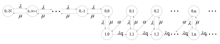
1.   Introduction

Throughout this paper, $\mathcal{H}$ denotes a real Hilbert space with inner product $\langle \cdot, \cdot\rangle$ and the induced $\|\cdot\|,$ $I$ the identity operator on $\mathcal{H},$ $\mathbb{N}$ the set of all natural numbers and $\mathbb{R}$ the set of all real numbers. For a self-operator $T$ on $\mathcal{H},$ $F(T)$ denotes the set of all fixed points of $T.$

Let $\mathcal{H}_1$ and $\mathcal{H}_2$ be real Hilbert spaces and let $\mathcal{T} : \mathcal{H}_1 \to \mathcal{H}_2$ be bounded linear operator. Let $\{U_j\}_{j = 1}^t: \mathcal{H}_1 \to \mathcal{H}_1$ and $\{T_i\}_{i = 1}^r: \mathcal{H}_2 \to \mathcal{H}_2$ be two finite families of operators, where $t, r\in \mathbb{N}.$ The split common fixed point problem (SCFPP) is formulated as finding a point $x^*\in \mathcal{H}_1$ such that

In particular, if $t = r = 1,$ the SCFPP (1.1) reduces to finding a point $x^*\in \mathcal{H}_1$ such that

The above problem is usually called the two-set SCFPP.

In recent years, the SCFPP (1.1) and the two-set SCFPP (1.2) have been studied and extended by many authors, see for instance ^{[15,20,23,27,36,37,38,39,40,47,48,49]}. It is known that the SCFPP includes the multiple-set split feasibility problem and split feasibility problem as a special case. In fact, let $\{C_j\}_{j = 1}^t$ and $\{Q_i\}_{i = 1}^r$ be two finite families of nonempty closed convex subsets in $\mathcal{H}_1$ and $\mathcal{H}_2,$ respectively. Let $U_j = P_{C_j}$ and $T_i = P_{Q_i};$ then SCFPP (1.1) becomes the multiple-set split feasibility problem (MSSFP) as follows:

When $t = r = 1$ the MSSFP (1.3) is reduced to the split feasibility problem (SFP) which is described as finding a point $x^*\in \mathcal{H}_1$ satisfying the following property

The SFP was first introduced by Censor and Elfving ^[22] with the aim of modeling certain inverse problems. It has turned out to also play an important role in, for example, medical image reconstruction and signal processing (see ^{[2,4,15,17,21]}). Since then, several iterative algorithms for solving (1.4) have been presented and analyzed. See, for instance ^{[1,5,14,15,16,18,19,23,24,27]} and references therein.

The $CQ$ algorithm has been extended by several authors to solve the multiple-set split convex feasibility problem. See, for instance, the papers by Censor and Segal ^[25], Elfving, Kopf and Bortfeld ^[23], Masad and Reich ^[35], and by Xu ^[53,54].

In 2020, Reich and Tuyen ^[45] proposed and analyzied the following split feasibility problem with multiple output sets in Hilbert spaces: let $\mathcal{H}, \mathcal{H}_i, i = 1, 2, \ldots, m$ be real Hilbert spaces. Let $\mathcal{T}_i: \mathcal{H} \to \mathcal{H}_i, \ i = 1, 2, \ldots, m,$ be bounded linear operators. Furthermore, let $C$ and $Q_i$ be nonempty, closed and convex subsets of $\mathcal{H}$ and $\mathcal{H}_i, i = 1, 2, \ldots, m,$ respectively. Find an element $u^{\dagger},$ such that:

that is, $u^\dagger \in C$ and $\mathcal{T}u^\dagger \in Q_i$, for all $i = 1, 2, \ldots, m.$

To solve problem (1.5), Reich et al. ^[46] proposed the following iterative methods: for any $u_0, v_0 \in C,$ let $\{u_n\}$ and $\{v_n\}$ be two sequence generated by:

where $f: C\to C$ is a strict $k$-contraction with $k\in [0, 1),$ $\{\gamma_n\} \subset (0, \infty)$ and $\{\alpha_n\} \subset (0, 1).$ They established the weak and strong convergence of iterative methods (1.6) and (1.7), respectively.

In 2021, Reich and Tuyen ^[44] considered the following split common null point problem with multiple output sets in Hilbert spaces: let $\mathcal{H}, \mathcal{H}_i, i = 1, 2, \ldots, N,$ be real Hilbert spaces and let $\mathcal{T}_i:\mathcal{H} \to \mathcal{H}_i, i = 1, 2, \ldots, N,$ be bounded linear operators. Let $\mathcal{B}: \mathcal{H} \to 2^{\mathcal{H}_i}, \; i = 1, 2, \ldots, N$ be maximal monotone operators. Given $\mathcal{H}, \mathcal{H}_i$ and $\mathcal{T}_i$ as defined above, the split common null point problem with multiple output sets is to find a point $u^\dagger$ such that

To solve problem (1.8), Reich and Tuyen ^[44] proposed the following iterative method:

Algorithm 1.1. For any $u_0\in \mathcal{H},$ Let $\mathcal{H}_0 = \mathcal{H}, \mathcal{T}_0 = I^{\mathcal{H}}, \mathcal{B}_0 = \mathcal{B},$ and let $\{u_n\}$ be the sequence generated by:

where $\{\alpha_n\} \subset (0, 1),$ and $\{\beta_{i, n}\}$ and $\{r_{i, n}\}, i = 0, 1, \ldots, N,$ are sequences of positive real numbers, such that $\{\beta_{i, n}\} \subset [a, b] \subset (0, 1)$ and $\sum_{i = 0}^{N}\beta_{i, n} = 1$ for each $n\geq 0,$ and $\tau_{i, n} = \rho_{i, n}\frac{\|(\mathcal{I}^{\mathcal{H}_i} - J_{r_{i, n}}^{\mathcal{B}_i})\mathcal{T}_iu_n\|^2}{\|\mathcal{T}_i^*(\mathcal{I}^{\mathcal{H}_i} - J_{r_{i, n}}^{\mathcal{B}_i})\mathcal{T}_iu_n\|^2 + \theta_{i, n}},$ where $\{\rho_{i, n}\} \subset [c, d] \subset (0, 2)$ and $\{\theta_{i, n}\}$ is a sequence of positive real numbers for each $i = 0, 1, \ldots, N,$ and $f:\mathcal{H} \to \mathcal{H}$ is a strict contraction mapping $\mathcal{H}$ into itself with the contraction coefficient $k\in [0, 1)$.

They established the strong convergence of the sequence $\{u_n\}$ generated by Algorithm 1.1 which is a solution of the Problem (1.8)

Alvarez and Attouch ^[7] applied the following inertial technique to develop an inertial proximal method for finding the zero of a monotone operator, i.e.,

where $G:H \to 2^H$ is a set-valued monotone operator. Given $x_{n-1},$ $x_n \in H$ and two parameters $\theta_n \in [0, 1),$ $\lambda_n > 0,$ find $x_{n+1} \in H$ such that

Here, the inertia is induced by the term $\theta_n(x_n - x_{n-1}).$ The equation (1.10) may be thought as coming from the implicit discretization of the second-other differential system

where $\rho > 0$ is a damping or a friction parameter. This point of view inspired various numerical methods related to the inertial terminology which has a nice convergence property ^{[6,7,8,28,29,33]} by incorporating second order information and helps in speeding up the convergence speed of an algorithm (see, e.g., ^{[3,7,9,10,11,12,13,51,52]} and the references therein).

Recently, Thong and Hieu ^[50] introduced an inertial algorithm to solve split common fixed point problem (1.1). The algorithm is of the form

Under approximate conditions, they show that the sequence $\{x_n\}$ generated by (1.12) converges weakly to some solution of SCFPP (1.1).

It was shown in [43, Section 4] by example that one-step inertial extrapolation $w_n = x_n + \theta(x_n - x_{n-1}), \ \theta\in [0, 1)$ may fail to provide acceleration. It was remarked in [32, Chapter 4] that the use of inertial of more than two points $x_n, x_{n-1}$ could provide acceleration. For example, the following two-step inertial extrapolation

with $\theta > 0$ and $\delta < 0$ can provide acceleration. The failure of one-step inertial acceleration of ADMM was also discussed in [42, Section 3] and adaptive acceleration for ADMM was proposed instead. Polyak ^[41] also discussed that the multi-step inertial methods can boost the speed of optimization methods even though neither the convergence nor the rate result of such multi-step inertial methods was established in ^[41]. Some results on multi-step inertial methods have recently be studied in ^[26].

Our Contributions. Motivated by ^[44,50], in this paper, we consider the following split common null point problem with multiple output sets in Hilbert spaces: Let $\mathcal{H}_1$ and $\mathcal{H}_2$ be real Hilbert spaces. Let $\{U_j\}_{j = 1}^r: \mathcal{H}_1\to \mathcal{H}_1$ be a finite family of quasi-nonexpansive operators and $\mathcal{B}_i: \mathcal{H}_2 \to 2^{\mathcal{H}_2}, i = 1, 2, \ldots, t.$ be maximal monotone operators and $\{\mathcal{T}_i\}_{i = 1}^t:\mathcal{H}_1 \to \mathcal{H}_2$ be a bounded linear operator. The split common null point problem with multiple output set is to find a point $x^*\in \mathcal{H}_1$ such that

Let $\Upsilon$ be the solution set of (1.14). We propose a two-step inertial extrapolation algorithm with self-adaptive step sizes for solving problem (1.14) and give the weak convergence result of our problem in real Hilbert spaces. We give numerical computations to show the efficiency of our proposed method.

2.   Preliminaries

Let $C$ be a nonempty, closed, and convex subset of a real Hilbert spaces $\mathcal{H}.$ We know that for each point $u^*\in \mathcal{H},$ there is a unique element $P_Cu^*\in C,$ such that:

We recall that the mapping $P_C:\mathcal{H}\to C$ defined by (2.1) is said to be metric projection of $\mathcal{H}$ onto $C.$ Moreover, we have (see, for instance, Section 3 in ^[31]):

Definition 2.1. Let $T:\mathcal{H} \to \mathcal{H}$ be an operator with $F(T) \neq \emptyset.$ Then

● $T: \mathcal{H} \to \mathcal{H}$ is called nonexpansive if

● $T:\mathcal{H} \to \mathcal{H}$ is quasi-nonexpansive if

We denote by $F(T)$ the set of fixed points of mapping $T;$ that is, $F(T) = \{u^*\in C : Tu^* = u^*\}.$ Given an operator $\mathcal{E}: \mathcal{H} \to 2^{\mathcal{H}},$ its domain, range, and graph are defined as follows:

and

The inverse operator $\mathcal{E}^{-1}$ of $\mathcal{E}$ is defined by:

Recall that the operator $\mathcal{E}$ is said to be monotone if, for each $u^*, v^*\in \mathcal{D}(\mathcal{E}),$ we have $\langle f-g, u^*-v^*\rangle \geq 0$ for all $f\in \mathcal{E}(u^*)$ and $g\in \mathcal{E}(v^*).$ We denote by $\mathcal{I}^{\mathcal{H}}$ the identity mapping on $\mathcal{H}.$ A monotone operator $\mathcal{E}$ is said to be maximal monotone if there is no proper monotone extension of $\mathcal{E}$ or, equivalently, by Minty's theorem, if $\mathcal{R}(\mathcal{I}^{\mathcal{H}} + \lambda\mathcal{E}) = \mathcal{H},$ for all $\lambda > 0.$ If $\mathcal{E}$ is maximal monotone, then we can define, for each $\lambda > 0,$ a nonexpansive single-valued operator $J_\lambda^{\mathcal{E}}: \mathcal{R}(\mathcal{I}^{\mathcal{H}} + \lambda \mathcal{E}) \to \mathcal{D}(\mathcal{E})$ by

This operator is called the resolvent of $\mathcal{E}.$ It is easy to see that $\mathcal{E}^{-1}(0) = F(J_\lambda^\mathcal{E})$, for all $\lambda > 0.$

Lemma 2.2. ^[45] Suppose that $\mathcal{E} :\mathcal{D}(\mathcal{E}) \subset \mathcal{H} \to 2^{\mathcal{H}}$ is a monotone operator. Then, we have the following statements:

(i) For $r\geq s > 0,$ we have:

for all elements $u\in \mathcal{R}(\mathcal{I}^{\mathcal{H}} + r\mathcal{E}) \cap \mathcal{R}(\mathcal{I}^{\mathcal{H}} + s\mathcal{E}).$

(ii) For all numbers $r > 0$ and for all points $u, v\in \mathcal{R}(\mathcal{I}^{\mathcal{H}} + r\mathcal{E}),$ we have:

(iii) For all numbers $r > 0$ and for all points $u, v\in \mathcal{R}(\mathcal{I}^{\mathcal{H}} + r\mathcal{E}),$ we have:

(iv) If $S = \mathcal{E}^{-1}(0) \neq \emptyset,$ then for all elements $u^*\in S$ and $u\in \mathcal{R}(\mathcal{I}^{\mathcal{H}} + r\mathcal{E}),$ we have:

Lemma 2.3. ^[30] Suppose that $\mathcal{T}$ is a nonexpansive mapping from a closed and convex subset of a Hilbert space $\mathcal{H}$ into $\mathcal{H}.$ Then, the mapping $\mathcal{I}^{\mathcal{H}} - \mathcal{T}$ is demiclosed on $\mathcal{C};$ that is, for any $\{u_n\} \subset \mathcal{C},$ such that $u_n \rightharpoonup u\in \mathcal{C}$ and the sequence $(\mathcal{I}^{\mathcal{H}} - \mathcal{T})(u_n) \to v,$ we have $(\mathcal{I}^{\mathcal{H}} - \mathcal{T})(u) = v.$

Lemma 2.4. ^[34] Given an integer $N\geq 1.$ Assume that for each $i = 1, \ldots, N$, $T_i:\mathcal{H} \to \mathcal{H}$ is a $k_i$-demicontractive operator such that $\cap_{i = 1}^NF(T_i) \neq \emptyset.$ Assume that $\{w_i\}_{i = 1}^N$ is a finite sequence of positive numbers such that $\sum_{i = 1}^{N}w_i = 1.$ Setting $U = \sum_{i = 1}^{N}w_iT_i,$ then the following results hold:

(i) $F(U) = \cap_{i = 1}^NF(T_i).$

(ii) $U$ is $\lambda$-demicontractive operator, where $\lambda = \max\{k_i|i = 1, \ldots, N\}.$

(iii) $\langle x -Ux, x -z\rangle \geq \frac{1-\lambda}{2}\sum_{i = 1}^{N}w_i\|x - T_ix\|^2$ for all $x\in \mathcal{H}$ and $z\in \cap_{i = 1}^NF(T_i).$

Lemma 2.5. Let $x, y, z\in \mathcal{H}$ and $\alpha, \beta \in \mathbb{R}.$ Then

3.   Main result

We give the following assumptions in order to obtain our convergence analysis.

Assumptions 3.1. We assume that the inertial parameters $\theta \in [0, \frac{1}{2}),$ $\rho \in (0, 1)$ and $\delta \in (-\infty, 0]$ satisfies the following conditions.

(a)

(b)

(c)

Now, we present our proposed method and our convergence analysis as follows:

Lemma 3.3. For $t\in \mathbb{N},$ let $\{\mathcal{B}_i\}_{i = 1}^t: \mathcal{H}_2 \to 2^{\mathcal{H}_2}$ be a finite family maximal monotone operators. Let $\{ T_i\}_{i = 1}^t: \mathcal{H}_1 \to \mathcal{H}_2,$ be a finite family of bounded linear operators. Define the operator $V: \mathcal{H}_1 \to \mathcal{H}_1$ by

where $\tau_{i, n}$ is as defined in (3.2), $\{\delta_{i, n}\}_{i = 1}^t \subset (0, 1)$ and $\sum_{i = 1}^{t}\delta_{i, n} = 1.$ Then we have the following results:

(1)

(2) $x\in F(V)$ if and only if $T_ix \in \cap_{i = 1}^tF(J_{r_{i, n}}^{\mathcal{B}_i})$, for $i = 1, 2, \ldots, t.$

Proof. (1) Given a point $z\in \Upsilon,$ it follows from the convexity of the function $\|\cdot\|^2$ that:

Using $J_{r_{i, n}}^{\mathcal{B}_i}(\mathcal{T}_iz) = \mathcal{T}_iz$ and Lemma 2.2(iii), for each $i = 1, 2, \ldots, t$, we see that

Hence, from (3.4) and (3.5), we get

(2) It is obvious that if $\mathcal{T}_ix \in \cap_{i = 1}^tF(J_{r_{i, n}}^{\mathcal{B}_i})$ then $x\in F(V).$ We show the converse, let $x\in F(V)$ and $z\in \mathcal{T}_i^{-1}\left(F(J_{r_{i, n}}^{\mathcal{B}_i})\right)$ we have

Since $\rho_{i, n} \subset (0, 2),$ we obtain

That is, $\mathcal{T}_ix \in \cap_{i = 1}^tF(J_{r_{i, n}}^{\mathcal{B}_i}).$

□

Lemma 3.4. For $t, r\in \mathbb{N},$ let $\{\mathcal{B}_i\}_{i = 1}^t: \mathcal{H}_2 \to \mathcal{H}_2$ be maximal monotone operators such that $\cap_{i = 1}^tF(J_{r_{i, n}}^{\mathcal{B}_i}) \neq \emptyset$ and $\{U_j\}_{j = 1}^r: \mathcal{H}_1 \to \mathcal{H}_1$ be a finite family of quasi-nonexpansive operators such that $\cap_{j = 1}^rF(U_j) \neq \emptyset.$ Assume that $\{\mathcal{I} - U_j\}_{j = 1}^r$ and $\{\mathcal{I} - J_{r_{i, n}}^{\mathcal{B}_i}\}_{i = 1}^t$ are demiclosed at zero. Let $\{\mathcal{T}_i\}_{i = 1}^t : \mathcal{H}_1 \to \mathcal{H}_2, \ $ be bounded linear operators suppose $\Upsilon \neq \emptyset.$ Let $S: \mathcal{H}_1 \to \mathcal{H}_1$ be defined by

where $\{\tau_{i, n}\},$ is as defined in (3.2), $\{w_j\}_{j = 1}^r$ and $\{\delta_{i, n}\}_{i = 1}^t$ are in $(0, 1)$ with $\sum_{j = 1}^{r}w_j = 1$ and $\sum_{i = 1}^{t}\delta_{i, n} = 1.$ Assume that the following conditions are satisfied

(A1) $\min_{i = 1, 2, \ldots, t}\{\inf_n\{r_{i, n}\}\} = r > 0;$

(A2) $\max_{i = 1, 2, \ldots, t}\{\sup_n\{\theta_{i, n}\}\} = K < \infty.$

Then the following hold:

(a) The operator $S$ is quasi-nonexpansive.

(b) $F(S) = \Upsilon$.

(c) $\mathcal{I} - S$ is demiclosed at zero.

Proof. From the definition of $V$ we can rewrite the operator $S$ as

We show the following

$({\rm{i}})$ $\{U_jV\}_{j = 1}^r$ is a finite family of quasi-nonexpansive operator,

$({\rm{ii}})$ $\cap_{j = 1}^rF(U_jV) = \Upsilon,$

$({\rm{iii}})$ for each $j = 1, 2, \ldots, r$ then $\mathcal{I} - U_jV$ is demiclosed at zero.

By Lemma 3.3, $V$ is quasi-nonexpansive. Therefore, for each $j = 1, 2, \ldots, r$ the operator $U_jV$ is quasi-nonexpansive. Next, we show that for each $j = 1, 2, \ldots, r,$ then

Indeed, it suffices to show that for each $j = 1, 2, \ldots, r$ $F(U_jV) \subset F(U_j) \cap F(V).$ Let $p\in F(U_jV).$ It is enough to show that $p\in F(V).$ Now, taking $z\in F(U_j) \cap F(V);$ we have

This implies that

That is $J_{r_{i, n}}^{\mathcal{B}_i}(\mathcal{T}_ip) = \mathcal{T}_ip, \ \ \ \forall \ \ i = 1, 2, \ldots, t.$ This implies that $\mathcal{T}_ip \in \cap_{i = 1}^tF(J_{r_{i, n}}^{\mathcal{B}_i}).$ Thus, $p\in F(V).$

Therefore, $F(U_j) \cap F(V) = F(U_jV), \ \ \forall j = 1, \ldots, r.$ We now show that

By Lemma 3.3, we have

Finally, we show that for each $j = 1, ..r,$ $\mathcal{I} - U_jV$ is demiclosed at zero. Let $\{x_n\} \subset \mathcal{H}_1$ be a sequence such that $x_n \rightharpoonup z \in \mathcal{H}_1$ and $U_jVx_n - x_n \to 0$ we have

This implies that

By Lemma 3.3, we have

This implies that

Since $\{\delta_{i, n}\} \subset [a, b] \subset (0, 1),$ $\{\rho_{i, n}\} \subset [c, d] \subset (0, 2),$ and (3.7) implies

$\forall \ \ \ i = 0, 1, 2\ldots t.$ It follows from the boundedness of the sequence $\{x_n\}$ that $L: = max_{i = 0, 1, \ldots, N}\{\sup\{\|\mathcal{T}_i^*(\mathcal{I}^{\mathcal{H}_2} - J_{r_{i, n}}^{\mathcal{B}_i})\mathcal{T}_ix_n\|^2\}\} < \infty.$ Thus from Condition (A2), It follows that

Combining this with (3.8), we deduce that

$\forall \ i = 0, 1, \ldots, N,$ Lemma 2.2(i) and Condition (A1) now imply that

$\forall \ i = 0, 1, \ldots, N.$ Thus using (3.9) and (3.10), we are able to deduce that

$\forall i = 0, 1, \ldots, N.$

From $\|Vx_n - x_n\| = \|\sum_{i = 0}^{t}\delta_{i, n}\tau_{i, n}\mathcal{T}_i^*(\mathcal{I}^{\mathcal{H}_2} - J_{r_{i, n}}^{\mathcal{B}_i})\mathcal{T}_ix_n\|,$ the assumptions on $\{\delta_{i, n}\}$ and $\{\tau_{i, n}\}$ and (3.10), it follows that

On the other hand

Since $x_n \rightharpoonup z,$ we have $Vx_n \rightharpoonup z$ and by the demiclosedness of $U_j$ we have $z\in F(U_j).$ Since, for each $i = 1, 2, \ldots, N,$ $\mathcal{T}_i$ is a bounded linear operator, it follows that $\mathcal{T}_ix_{n_k} \rightharpoonup \mathcal{T}_iz.$ Thus by Lemma 2.3 and (3.11) implies that $\mathcal{T}_iz \in F(J_r^{\mathcal{B}_i}) \ \ \forall i = 1, \ldots, t$ that is $\mathcal{T}_iz \in \cap_{i = 1}^tF(J_r^{\mathcal{B}_i}).$ By Lemma 3.3 we get $z\in F(V).$ Therefore, $z\in F(U_j)\cap F(V) = F(U_jV).$

By Claim (i) and Lemma 2.4, we obtain $Sx = \sum_{j = 1}^{r}w_jU_jVx$ is quasi-nonexpansive and $F(S) = \cap_{j = 1}^tF(U_jV) = \Upsilon.$

Finally, we show that $\mathcal{I} - S$ is demiclosed at zero. Indeed, Let $\{x_n\}\subset \mathcal{H}_1$ be a sequence such that $x_n \rightharpoonup z\in \mathcal{H}_1$ and $\|x_n - Sx_n\| \to 0.$ Let $p\in F(S)$ by Lemma 2.4, we have

This imples that, for each $j = 1, \ldots, t$ we have

By the demiclosedness of $\mathcal{I} - U_jV$ we have $z\in F(U_jV).$ Therefore $z\in \cap_{j = 1}^tF(U_jV) = F(S).$ □

Theorem 3.5. For $t, r\in \mathbb{N}.$ Let $\{\mathcal{B}_i\}_{i = 1}^t: \mathcal{H}_2 \to \mathcal{H}_2$ be a finite family of maximal monotone operators such that $\cap_{i = 1}^tF(J_r^{\mathcal{B}_i})\neq \emptyset$ and $\{U_j\}_{j = 1}^r:\mathcal{H}_1 \to \mathcal{H}_1$ be a finite family of quasi-nonexpansive operators such that $\cap_{j = 1}^rF(U_j) \neq \emptyset.$ Assume that $\{\mathcal{I} - U_j\}_{j = 1}^r$ and $\{\mathcal{I} - J_r^{\mathcal{B}_i}\}_{i = 1}^t$ are demiclosed at zero. Let $\mathcal{T}_i:\mathcal{H}_1 \to \mathcal{H}_2,$ $i = 1, 2, \ldots, N$ be bounded linear operators. Suppose $\Upsilon \neq \emptyset.$ Let $\{x_n\}$ be a sequence generated by Algorithm 3.2. and suppose that Assumptions (3.1) (a)-(c) are fulfilled. Then $\{x_n\}$ converges weakly to an element of $\Upsilon.$

Proof. Let $S = \sum_{j = 1}^{r}w_jU_j\left(\mathcal{I} - \sum_{i = 1}^{t}\delta_{i, n}\tau_{i, n}\mathcal{T}_i^*(\mathcal{I}^{\mathcal{H}_2} - J_{r_{i, n}}^{\mathcal{B}_i})\mathcal{T}_i\right),$ then the sequence $\{x_{n+1}\}$ can be rewritten as follows

By Lemma 3.3, we have that $S$ is quasi-nonexpansive. Let $z\in \Upsilon,$ from (3.13), we get

Observe that

Hence by Lemma 2.5, we have

Note also that

and so,

Also,

which implies that

Similarly, we have

and thus

By (3.16)–(3.18) and Cauchy-Schwartz inequality one has

Observe that

Putting (3.20) in (3.14), we get

Combining (3.15) and (3.19) in (3.21) with noting that $\delta \leq 0$ we obtain

By rearranging we get

Define

Let us show that $\Upsilon_n \geq 0, \forall n\geq 1.$ Now

Since $\theta < 1/2,$ $\delta \leq 0,$ $\frac{2\theta\rho}{1-\rho} - (1-\theta) < \delta$ and $0\leq \theta < \frac{1-\rho}{1+\rho},$ it follows from (3.24) that $\Upsilon_n \geq 0.$ Furthermore, we drive from (3.23)

where

and

By our assumption, it holds that

As a result $q_1 > 0.$ Also $q_2 > 0$ by Assumption 3.1 (c). Then by (3.25) we have

Letting $\bar{\Upsilon}_n: = \Upsilon_n + q_1\|x_{n-1} - x_{n-2}\|^2.$ Then $\bar{\Upsilon}_n \geq 0, \ \forall n\geq 1.$ Also, it follows from (3.28) that

These facts imply that the sequence $\{\bar{\Upsilon}_n\}$ is decreasing and bounded from below and thus $\underset{n\to \infty}\lim\bar{\Upsilon}_n$ exists. Consequently, we get from (3.28) and the squeeze theorem that

Hence

As a result

as $n\to \infty.$ By $\underset{n\to \infty}\lim\|x_{n+1} - x_n\| = 0$, one has

By (3.31) and the existence of $\underset{n\to \infty}\lim\bar{\Upsilon}_n,$ we have that $\underset{n\to \infty}\lim\Upsilon_n$ exists and hence $\{\Upsilon_n\}$ is bounded. Now, since $\underset{n\to \infty}\lim\|x_{n+1} - x_n\| = 0,$ we have from the definition of $\Upsilon_n$ that

exists. Using the boundedness of $\{\Upsilon_n\},$ we obtain from (3.24) that $\{x_n\}$ is bounded. Consequently $\{y_n\}$ is bounded. From (3.8), we obtain

This implies that

Finally, we show that the sequence $\{x_n\}$ converges weakly to $x^*\in \Upsilon.$ Indeed, since $\{x_n\}$ is bounded we assume that there exists a subsequence $\{x_{n_j}\}$ of $\{x_n\}$ such that $x_{n_j} \rightharpoonup x^*\in H.$ Since $\|x_n - y_n\| \to 0,$ we also have $y_{n_j} \rightharpoonup x^*$. Then by the demiclosedness of $I-S$, we obtain $x^*\in F(S) = \Upsilon.$

Now, we show that $\{x_n\}$ has unique weak limit point in $\Upsilon.$ Suppose that $\{x_{m_j}\}$ is another subsequence of $\{x_n\}$ such that $x_{m_j} \rightharpoonup v^*$ as $j\to \infty$. Observe that

and

Therefore

and

Addition of (3.34)–(3.36) gives

According to (3.32), we get

exists and

exists. This implies from (3.21) that $\underset{n\to \infty}\lim \langle x_{n} - \theta x_{n-1} - \delta x_{n-2}, x^* - v^*\rangle$ exists. Consequently,

Hence

Since $\delta \leq 0 < 1-\theta,$ we obtain that $x^* = v^*.$ Therefore, the sequence $\{x_n\}$ converges weakly to $x^*\in \Upsilon.$ This completes the proof. □

4.   Numerical examples

In this section, we give a numerical description to illustrate how our proposed algorithm can be implemented in the setting of the real Hilbert space $\mathbb{R}$. Furthermore, we shall show the effect of the double inertia in the fast convergence of the sequence generated by our proposed Algorithm 3.2. First, we give the set of parameters that satisfy the conditions given in assumption 3.1. To this end, fix $\rho = \frac{1}{2}$ and take

Clearly, these parameters satisfy the conditions given in assumption 3.1. Next, we define the operators to be used in the implementation of Algorithm 3.2. In Algorithm 3.2, fix $t = N = r = 3$. Set $H_1 = H_2 = H_3 = \mathbb{R}.$ Let $\delta_{i, n} = \frac{1}{3}$, $\rho_{i, n} = \theta_{i, n} = \frac{2}{3}$, $r_{i, n} = \frac{1}{2}$ and $w_j = \frac{1}{3}$, where $i, j\in\{1, 2, 3\}$ and $n\geq 1$. Let $B_i, \; T_i, \; U_j :\mathbb{R} \to \mathbb{R}$ be defined by

Then,

With this, we are ready to implement our proposed Algorithm 3.2 on MATLAB. Choosing $x_0 = 1, \; x_1 = -2$ and $x_2 = 0.5$, and setting maximum number of iterations to 150 or $10^{-16}$, as our stopping criteria, we varied the double inertial parameters as given above. We obtained the following successive approximations:

5.   Discussion

From the numerical simulations presented in Table 1 and Figures 1–3, we saw that in this example, the best choice for the double inertial parameters is $\theta = \frac{1}{4}$ and $\delta = -\frac{1}{1000}$. Furthermore, we observed that as $\theta$ decreases and $\delta$ approaches $0$, the number of iterations required to satisfy the stopping criteria increases.

Use of AI tools declaration

The authors declare they have not used Artificial Intelligence (AI) tools in the creation of this article.

Acknowledgments

This research was supported by The Science, Research and Innovation Promotion Funding (TSRI) [grant number FRB660012/0168]. This research block grants was managed under Rajamangala University of Technology Thanyaburi [grant number FRB66E0628].

Conflict of interest

All authors declare no conflicts of interest in this paper.