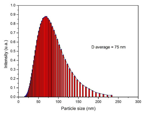
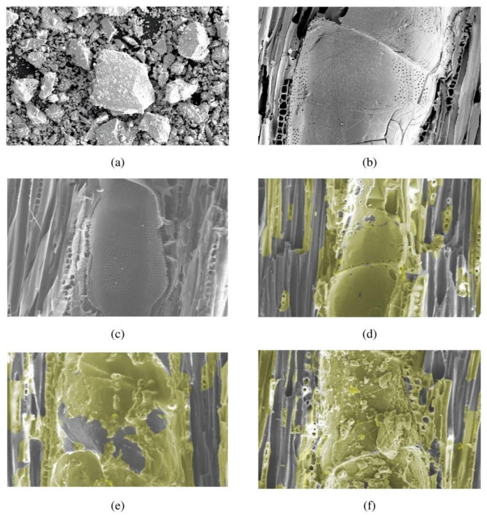
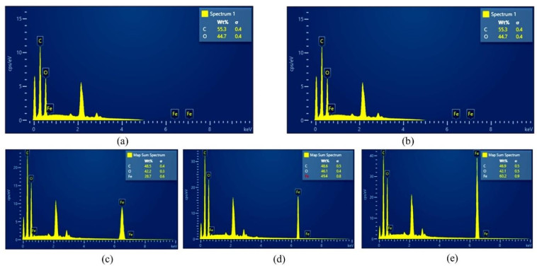
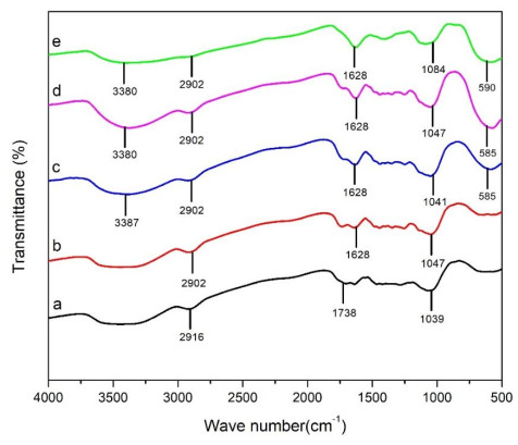
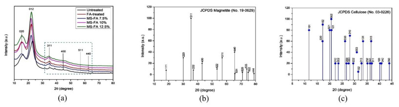
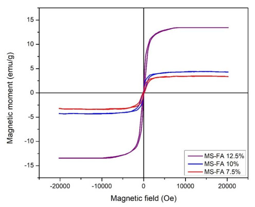
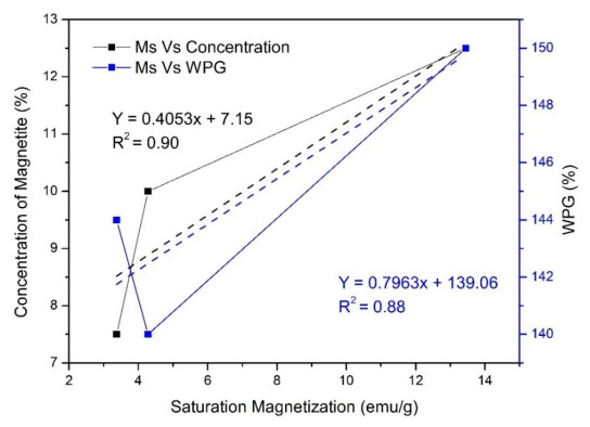
This study was conducted to synthesize magnetic wood through the ex situ impregnation method of magnetite nanoparticles and analyze its physical properties and characterization. The process was initiated with the synthesis of magnetite nanoparticles by the co-precipitation method and the nano-magnetite was successfully synthesized with a particle distribution of 17–233 nm at an average size of 75 nm. Furthermore, the impregnation solution consisted of three different levels of magnetite nanoparticles dispersed in furfuryl alcohol, untreated and furfurylated wood for comparison. Sengon wood (Falcataria moluccana Miq.) was also used due to its low physical properties. The impregnation process was conducted by immersing the samples in the solution at a vacuum of −0.5 bar for 30 min, followed by a pressure of 1 bar for 2 h. There was also an improvement in the physical properties, such as weight percent gain, bulking effect, anti-swelling efficiency and density, while the water uptake continued to decrease. Additionally, magnetite nanoparticles appeared in wood microstructure image, supported by the result of ferrum content in chemical element analysis. The results showed that chemical change analysis proved the presence of Fe–O functional group cross-linked with wood polymer. The diffractogram also reported the appearance of magnetite nanoparticles peak and a decrease in crystallinity due to an increase in the concentration. Based on the analysis, sengon wood was classified as a superparamagnetic material with soft magnetic characteristics and the optimum treatment was furfurylated-magnetite 12.5% wood.
Citation: Saviska Luqyana Fadia, Istie Rahayu, Deded Sarip Nawawi, Rohmat Ismail, Esti Prihatini, Gilang Dwi Laksono, Irma Wahyuningtyas. Magnetic characteristics of sengon wood-impregnated magnetite nanoparticles synthesized by the co-precipitation method[J]. AIMS Materials Science, 2024, 11(1): 1-27. doi: 10.3934/matersci.2024001
This study was conducted to synthesize magnetic wood through the ex situ impregnation method of magnetite nanoparticles and analyze its physical properties and characterization. The process was initiated with the synthesis of magnetite nanoparticles by the co-precipitation method and the nano-magnetite was successfully synthesized with a particle distribution of 17–233 nm at an average size of 75 nm. Furthermore, the impregnation solution consisted of three different levels of magnetite nanoparticles dispersed in furfuryl alcohol, untreated and furfurylated wood for comparison. Sengon wood (Falcataria moluccana Miq.) was also used due to its low physical properties. The impregnation process was conducted by immersing the samples in the solution at a vacuum of −0.5 bar for 30 min, followed by a pressure of 1 bar for 2 h. There was also an improvement in the physical properties, such as weight percent gain, bulking effect, anti-swelling efficiency and density, while the water uptake continued to decrease. Additionally, magnetite nanoparticles appeared in wood microstructure image, supported by the result of ferrum content in chemical element analysis. The results showed that chemical change analysis proved the presence of Fe–O functional group cross-linked with wood polymer. The diffractogram also reported the appearance of magnetite nanoparticles peak and a decrease in crystallinity due to an increase in the concentration. Based on the analysis, sengon wood was classified as a superparamagnetic material with soft magnetic characteristics and the optimum treatment was furfurylated-magnetite 12.5% wood.

| [1] |
Mashkour M, Ranjbar Y (2018) Superparamagnetic Fe3O4@ wood flour/polypropylene nanocomposites: Physical and mechanical properties. Ind Crop Prod 111: 47–54. https://doi.org/10.1016/j.indcrop.2017.09.068 doi: 10.1016/j.indcrop.2017.09.068

|
| [2] |
Sudirman AW (2020) Effect of cellphone electromagnetic wave radiation on the development of sperm. JIKSH 9: 708–712. https://doi.org/10.35816/jiskh.v12i2.385 doi: 10.35816/jiskh.v12i2.385
|
| [3] | Swamardika IBA (2009) Pengaruh radiasi gelombang elektromagnetik terhadap kesehatan manusia (suatu kajian pustaka). MITE 8: 1–4. https://ojs.unud.ac.id/index.php/jte/article/view/1585 |
| [4] |
Wang S, Ashfaq MZ, Gong H, et al. (2021) Electromagnetic wave absorption properties of magnetic particle-doped SiCN (C) composite ceramics. J Mater Sci Mater Electron 32: 4529–4543. https://doi.org/10.1007/s10854-020-05195-5 doi: 10.1007/s10854-020-05195-5
|
| [5] |
Gao K, Zhao J, Bai Z, et al. (2019) The preparation of FeCo/ZnOcomposites and enhancement of microwave absorbing property by two-step method. Materials 12: 3259. https://doi.org/10.3390/ma12193259 doi: 10.3390/ma12193259
|
| [6] |
Lu C, Wu M, Lin L, et al. (2019) Single-phase multiferroics: New materials, phenomena, and physics. Natl Sci Rev 6: 653–668. https://doi.org/10.1093/nsr/nwz091 doi: 10.1093/nsr/nwz091
|
| [7] |
Zhao Z, Gao Z, Lan D, et al. (2021) MOFs-derived hollow materials for electromagnetic wave absorption: Prospects and challenges. J Mater Sci Mater Electron 32: 25631–25648. https://doi.org/10.1007/s10854-021-06069-0 doi: 10.1007/s10854-021-06069-0
|
| [8] |
Shanenkov I, Sivkov A, Ivashutenko A, et al. (2017) Magnetite hollow microspheres with a broad absorption bandwidth of 11.9 GHz: Toward promising lightweight electromagnetic microwave absorption. Phys Chem Chem Phys 19: 19975–19983. https://doi.org/10.1039/c7cp03292g doi: 10.1039/c7cp03292g
|
| [9] |
Wang F, Liu J, Kong J, et al. (2011) Template free synthesis and electromagnetic wave absorption properties of monodispersed hollow magnetite nano-spheres. J Mater Chem 21: 4314–4320. https://doi.org/10.1039/c0jm02894k doi: 10.1039/c0jm02894k
|
| [10] |
Zhang D, Cheng J, Yang X (2014) Electromagnetic and microwave absorbing properties of magnetite nanoparticles decorated carbon nanotubes/polyaniline multiphase heterostructures. J Mater Sci 49: 7221–7230. https://doi.org/10.1007/s10853-014-8429-3 doi: 10.1007/s10853-014-8429-3
|
| [11] |
Lou Z, Li Y, Han H, et al. (2018) Synthesis of porous 3D Fe/C composites from waste wood with tunable and excellent electromagnetic wave absorption performance. ACS Sustainable Chem Eng 6: 15598–15607. https://doi.org/10.1021/acssuschemeng.8b04045 doi: 10.1021/acssuschemeng.8b04045
|
| [12] |
Lou Z, Han H, Zhou M, et al. (2018) Synthesis of magnetic wood with excellent and tunable electromagnetic wave-absorbing properties by a facile vacuum/pressure impregnation method. ACS Sustainable Chem Eng 6: 1000–1008. https://doi.org/10.1021/acssuschemeng.7b03332 doi: 10.1021/acssuschemeng.7b03332
|
| [13] |
Zhao S, Gao Z, Chen C, et al. (2016) Alternate nonmagnetic and magnetic multilayer nanofilms deposited on carbon nanocoils by atomic layer deposition to tune microwave absorption property. Carbon 98: 196–203. https://doi.org/10.1016/j.carbon.2015.10.101 doi: 10.1016/j.carbon.2015.10.101
|
| [14] |
Qiang R, Du Y, Wang Y, et al. (2016) Rational design of yolk-shell C@C microspheres for the effective enhancement in microwave absorption. Carbon 98: 599–606. https://doi.org/10.1016/j.carbon.2015.11.054 doi: 10.1016/j.carbon.2015.11.054
|
| [15] |
Xu H, Yin X, Zhu M, et al. (2017) Carbon hollow microspheres with a designable mesoporous shell for high-performance electromagnetic wave absorption. ACS Appl Mater Interfaces 9: 6332–6341. https://doi.org/10.1021/acsami.6b15826 doi: 10.1021/acsami.6b15826
|
| [16] |
Zhang N, Huang Y, Wang M (2018) 3D ferromagnetic graphene nanocomposites with ZnO nanorods and Fe3O4 nanoparticles co-decorated for efficient electromagnetic wave absorption. Compos Part B-Eng 136: 135–142. https://doi.org/10.1016/j.compositesb.2017.10.029 doi: 10.1016/j.compositesb.2017.10.029
|
| [17] |
Zhang H, Xie A, Wang C, et al. (2013) Novel rGO/α-Fe2O3 composite hydrogel: Synthesis, characterization and high performance of electromagnetic wave absorption. J Mater Chem A 1: 8547–8552. https://doi.org/10.1039/c3ta11278k doi: 10.1039/c3ta11278k
|
| [18] |
Zhang N, Huang Y, Zong M, et al. (2017) Synthesis of ZnS quantum dots and CoFe2O4 nanoparticles co-loaded with graphene nanosheets as an efficient broad band EM wave absorber. Chem Eng J 308: 214–221. https://doi.org/10.1016/j.cej.2016.09.065 doi: 10.1016/j.cej.2016.09.065
|
| [19] |
Trey S, Olsson RT, Ström V, et al. (2014) Controlled deposition of magnetic particles within the 3-D template of wood: Making use of the natural hierarchical structure of wood. RSC Adv 4: 35678–35685. https://doi.org/10.1039/c4ra04715j doi: 10.1039/c4ra04715j
|
| [20] |
Gan W, Gao L, Zhan X, et al. (2015) Hydrothermal synthesis of magnetic wood composites and improved wood properties by precipitation with CoFe2O4/hydroxyapatite. RSC Adv 5: 45919–45927. https://doi.org/10.1039/c5ra06138e doi: 10.1039/c5ra06138e
|
| [21] |
Lou Z, Zhang Y, Zhou M, et al. (2018) Synthesis of magnetic wood fiber board and corresponding multi-layer magnetic composite board, with electromagnetic wave absorbing properties. Nanomaterials 8: 1–14. https://doi.org/10.3390/nano8060441 doi: 10.3390/nano8060441
|
| [22] |
Liu TT, Cao MQ, Fang YS, et al. (2022) Green building materials lit up by electromagnetic absorption function: A review. J Mater Sci Technol 112: 329–344. https://doi.org/10.1016/j.jmst.2021.10.022 doi: 10.1016/j.jmst.2021.10.022
|
| [23] |
Lou Z, Han X, Liu J, et al. (2021) Nano-Fe3O4/bamboo bundles/phenolic resin oriented recombination ternary composite with enhanced multiple functions. Compos Part B-Eng 226: 109335. https://doi.org/10.1016/J.COMPOSITESB.2021.109335 doi: 10.1016/j.compositesb.2021.109335
|
| [24] |
Oka H, Terui M, Osada H, et al. (2012) Electromagnetic wave absorption characteristics adjustment method of recycled powder-type magnetic wood for use as a building material. IEEE Trans Magn 48: 3498–3500. https://doi.org/10.1109/TMAG.2012.2196026 doi: 10.1109/TMAG.2012.2196026
|
| [25] |
Pourjafar S, Rahimpour A, Jahanshahi M (2012) Synthesis and characterization of PVA/PES thin film composite nanofiltration membrane modified with TiO2 nanoparticles for better performance and surface properties. J Ind Eng Chem 18: 1398–1405. https://doi.org/10.1016/j.jiec.2012.01.041 doi: 10.1016/j.jiec.2012.01.041
|
| [26] |
Oka H, Fujita H (1999) Experimental study on magnetic and heating characteristics of magnetic wood. J Appl Phys 85: 5732–5734. https://doi.org/10.1063/1.370267 doi: 10.1063/1.370267
|
| [27] |
Dong Y, Yan Y, Zhang S, et al. (2014) Wood/polymer nanocomposites prepared by impregnation with furfuryl alcohol and Nano-SiO2. BioResources 9: 6028–6040. https://doi.org/10.15376/biores.9.4.6028-6040 doi: 10.15376/biores.9.4.6028-6040
|
| [28] |
Rahayu I, Prihatini E, Ismail R, et al. (2022) Fast-growing magnetic wood synthesis by an in-situ method. Polymers 14: 2137. https://doi.org/10.3390/polym14112137 doi: 10.3390/polym14112137
|
| [29] |
Zhang X, Zhou R, Rao W, et al. (2006) Influence of precipitator agents NaOH and NH4OH on the preparation of Fe3O4 nano-particles synthesized by electron beam irradiation. J Radioanal Nucl Chem 270: 285–289. https://doi.org/10.1007/s10967-006-0346-8 doi: 10.1007/s10967-006-0346-8
|
| [30] |
Fajriani E, Ruelle J, Dlouha J, et al. (2013) Radial variation of wood properties of sengon (paraserianthes falcataria) and jabon (anthocephalus cadamba). J Indian Acad Wood Sci 10: 110–117. https://doi.org/10.1007/s13196-013-0101-z doi: 10.1007/s13196-013-0101-z
|
| [31] | Rahayu I, Darmawan W, Nugroho N, et al. (2014) Demarcation point between juvenile and mature wood in sengon (falcataria moluccana) and jabon (antocephalus cadamba). J Trop For Sci 26: 331–339. https://www.jstor.org/stable/43150914 |
| [32] |
Priadi T, Sholihah M, Karlinasari L (2019) Water absorption and dimensional stability of heat-treated fast-growing hardwoods. J Korean Wood Sci Technol 47: 567–578. https://doi.org/10.5658/WOOD.2019.47.5.567 doi: 10.5658/WOOD.2019.47.5.567
|
| [33] |
Hadi YS, Massijaya MY, Abdillah IB, et al. (2020) Color change and resistance to subterranean termite attack of mangium (acacia mangium) and sengon (falcataria moluccana) smoked wood. J Korean Wood Sci Technol 48: 1–11. https://doi.org/10.5658/WOOD.2020.48.1.1 doi: 10.5658/WOOD.2020.48.1.1
|
| [34] | Hartati N, Sudarmonowati E, Fatriasari W, et al. (2010) Wood characteristic of superior sengon collection and prospect of wood properties improvement through genetic engineering. Wood Res J 1: 103–107. https://api.semanticscholar.org/CorpusID:89700771 |
| [35] | Krisnawati H, Kallio M, Kanninen M (2011) Anthocephalus Cadamba Miq.: Ecology, Silviculture and Productivity, Bogor: Center for International Forestry Research. https://doi.org/10.17528/cifor/003481 |
| [36] |
Laksono GD, Rahayu IS, Karlinasari L, et al. (2023) Characteristics of magnetic sengon wood impregnated with nano Fe3O4 and furfuryl alcohol. J Korean Wood Sci Technol 51: 1–13. https://doi.org/10.5658/WOOD.2023.51.1.1 doi: 10.5658/WOOD.2023.51.1.1
|
| [37] |
Jaunslavietis J, Shulga G, Ozolins J, et al. (2018) Hydrophilic-hydrophobic characteristics of wood-polymer composites filled with modified wood particle. Key Eng Mater 762: 176–181. https://doi.org/10.4028/www.scientific.net/KEM.762.176 doi: 10.4028/www.scientific.net/KEM.762.176
|
| [38] |
Prihatini E, Wahyuningtyas I, Rahayu I, et al. (2022) Modification of fast-growing wood into magnetic wood with impregnation method using Fe3O4 nanoparticles. J Sylva Lestari 10: 211–222. https://doi.org/10.23960/jsl.v11i2.651 doi: 10.23960/jsl.v11i2.651
|
| [39] |
Tathod AP, Dhepe PL (2015) Efficient method for the conversion of agricultural waste into sugar alcohols over supported bimetallic catalysts. Bioresource Technol 178: 36–44. https://doi.org/10.1016/j.biortech.2014.10.036 doi: 10.1016/j.biortech.2014.10.036
|
| [40] |
Teng TJ, Arip MNM, Sudesh K, et al. (2018) Conventional technology and nanotechnology in wood preservation: A review. BioResources 13: 9220–9252. https://doi.org/10.15376/biores.13.4.Teng doi: 10.15376/biores.13.4.Teng
|
| [41] |
Baysal E, Ozaki SK, Yalinkilic MK (2004) Dimensional stabilization of wood treated with furfuryl alcohol catalysed by borates. Wood Sci Technol 38: 405–415. https://doi.org/10.1007/s00226-004-0248-2 doi: 10.1007/s00226-004-0248-2
|
| [42] |
Dong Y, Yan Y, Zhang Y, et al. (2016) Combined treatment for conversion of fast-growing poplar wood to magnetic wood with high dimensional stability. Wood Sci Technol 50: 503–517. https://doi.org/10.1007/s00226-015-0789-6 doi: 10.1007/s00226-015-0789-6
|
| [43] |
Li F, Jiang S, Huang J, et al. (2019) Catalytic transfer hydrogenation of furfural to furfuryl alcohol over a magnetic Fe3O4@C catalyst. New J Chem 44: 478–486. https://doi.org/10.1039/c9nj04698d doi: 10.1039/c9nj04698d
|
| [44] |
Hou P, Ma M, Zhang P, et al. (2021) Catalytic transfer hydrogenation of furfural to furfuryl alcohol using easy-to-separate core–shell magnetic zirconium hydroxide. New J Chem 45: 2715–2722. https://doi.org/10.1039/d0nj05638c doi: 10.1039/d0nj05638c
|
| [45] |
Alibegovic K, Morgan G, Losovyj Y, et al. (2017) Efficient furfuryl alcohol synthesis from furfural over magnetically recoverable catalysts: Does the catalyst stabilizing medium matter? ChemistrySelect 2: 5485–5491. https://doi.org/10.1002/slct.201701100 doi: 10.1002/slct.201701100
|
| [46] |
Wahyuningtyas I, Rahayu IS, Maddu A, et al. (2022) Magnetic properties of wood treated with nano-magnetite and furfuryl alcohol impregnation. BioResources 17: 6496–6510. https://ojs.cnr.ncsu.edu/index.php/BRJ/article/view/22098 doi: 10.15376/biores.17.4.6496-6510
|
| [47] |
Cheng Z, Wei Y, Liu C, et al. (2020) Lightweight and construable magnetic wood for electromagnetic interference shielding. Adv Eng Mater 22: 1–24. https://doi.org/10.1002/adem.202000257 doi: 10.1002/adem.202000257
|
| [48] |
Zheng Y, Song Y, Gao T, et al. (2020) Lightweight and hydrophobic three-dimensional wood-derived anisotropic magnetic porous carbon for highly efficient electromagnetic interference shielding. ACS Appl Mater Interfaces 12: 40802–40814. https://doi.org/10.1021/acsami.0c11530 doi: 10.1021/acsami.0c11530
|
| [49] | British Standard (1957) Methods of Testing Small Clear Specimens of Timber, London: British Standard Institution. Available from: https://allcivilstandard.com/wp-content/uploads/2019/02/BS-00373-1957-1999.pdf. |
| [50] |
Peternele WS, Monge Fuentes V, Fascineli ML, et al. (2014) Experimental investigation of the coprecipitation method: An approach to obtain magnetite and maghemite nanoparticles with improved properties. J Nanomater 2014: 682985. https://doi.org/10.1155/2014/682985 doi: 10.1155/2014/682985
|
| [51] | Cornell RM, Schwertmann U (2003) The Iron Oxides: Structure, Properties, Reactions, Occurencs and Uses, Weinheim: Wiley. https://doi.org/10.1002/3527602097 |
| [52] |
Sompech S, Srion A, Nuntiya A (2012) The effect of ultrasonic treatment on the particle size and specific surface area of LaCoO3. Procedia Eng 32: 1012–1018. https://doi.org/10.1016/j.proeng.2012.02.047 doi: 10.1016/j.proeng.2012.02.047
|
| [53] |
Oka H, Fujita H, Seki K (2000) Composition and heating efficiency of magnetic wood by induction heating. IEEE Trans Magn 36: 3715–3717. https://doi.org/10.1109/20.908950 doi: 10.1109/20.908950
|
| [54] | Bowyer JL, Shmulsky R, Haygreen JG (2007) Forest Products and Wood Science—An Introduction, Iowa: Blackwell Publisher. https://doi.org/10.1002/9780470960035 |
| [55] | Rowell RM, Ellis WD (1978) Determination of dimensional stabilization of wood using the water-soak method. Wood Fiber Sci 10: 104–111. https://wfs.swst.org/index.php/wfs/article/view/1004 |
| [56] | Hill CAS (2006) Wood Modification: Chemical, Thermal, and Other Processes, West Sussex: Willey. https://doi.org/10.1002/0470021748 |
| [57] |
Gerasimov AM, Eremina OV, Cherkasova MV, et al. (2021) Application of particle-size analysis in various industries. J Phys Conf Ser 1728: 012003. https://doi.org/10.1088/1742-6596/1728/1/012003 doi: 10.1088/1742-6596/1728/1/012003
|
| [58] |
Jayaprakash J, Srinivasan N, Chandrasekaran P (2014) Surface modifications of CuO nanoparticles using ethylene diamine tetra acetic acid as a capping agent by sol-gel routine. Spectrochim Acta A 123: 363–368. https://doi.org/10.1016/J.SAA.2013.12.080 doi: 10.1016/j.saa.2013.12.080
|
| [59] |
Dubey V, Kain V (2018) Synthesis of magnetite by coprecipitation and sintering and its characterization. Mater Manuf Process 33: 835–839. https://doi.org/10.1080/10426914.2017.1401720 doi: 10.1080/10426914.2017.1401720
|
| [60] |
Fumis DB, Silveira MLDC, Gaglieri C, et al. (2022) The effect of EDTA functionalization on Fe3O4 thermal behavior. Mat Res 25: 1–6. https://doi.org/10.1590/1980-5373-MR-2022-0312 doi: 10.1590/1980-5373-MR-2022-0312
|
| [61] |
Magdalena AG, Silva IMB, Marques RFC, et al. (2018) EDTA-functionalized Fe3O4 nanoparticles. J Phys Chem Solids 113: 5–10. https://doi.org/10.1016/j.jpcs.2017.10.002 doi: 10.1016/j.jpcs.2017.10.002
|
| [62] |
Wang M, Wang N, Tang H, et al. (2012) Surface modification of nano-Fe3O4 with EDTA and its use in H2O2 activation for removing organic pollutants. Catal Sci Technol 2: 187–194. https://doi.org/10.1039/c1cy00260k doi: 10.1039/c1cy00260k
|
| [63] |
Pereira SV, Colombo FB, De Freitas LAP (2016) Ultrasound influence on the solubility of solid dispersions prepared for a poorly soluble drug. Ultrason Sonochem 29: 461–469. https://doi.org/10.1016/j.ultsonch.2015.10.022 doi: 10.1016/j.ultsonch.2015.10.022
|
| [64] |
Dudchenko N, Pawar S, Perelshtein I, et al. (2022) Magnetite nanoparticles: Synthesis and applications in optics. Materials 15: 2601. https://doi.org/10.3390/ma15072601 doi: 10.3390/ma15072601
|
| [65] |
Mascolo MC, Pei Y, Ring TA, et al. (2013) Room temperature co-precipitation synthesis of magnetite nanoparticles in a large pH window with different bases. Materials 6: 5549–5567. https://doi.org/10.3390/ma6125549 doi: 10.3390/ma6125549
|
| [66] |
Khan I, Saeed K, Khan I (2019) Nanoparticles: Properties, applications and toxicities. Arab J Chem 12: 908–931. https://doi.org/10.1016/j.arabjc.2017.05.011 doi: 10.1016/j.arabjc.2017.05.011
|
| [67] |
Fan S, Gao X, Pang J, et al. (2023) Enhanced preservative performance of pine wood through nano-xylan treatment assisted by high-temperature steam and vacuum impregnation. Materials 16: 3976. https://doi.org/10.3390/ma16113976 doi: 10.3390/ma16113976
|
| [68] |
Yulianingsih R, Sugiarto Y, Putranto W (2015) Mass transfer characteristics during vacuum impregnation process of papaya fruit in sucrose solution. JTP 16: 159–166. https://jtp.ub.ac.id/index.php/jtp/article/view/515 doi: 10.21776/ub.jtp.2015.016.03.01
|
| [69] | Martawijaya A, Hadjodarsono S, Haji M (2005) Atlas Kayu Indonesia, 2 Eds., Bogor: IAWA Journal. |
| [70] | Praptoyo H (2005) Comparative study of two types sampling method for measuring cell proportion and fiber dimension on sengon salomon wood. J Ilmu Teknologi Kayu Tropis 3: 60–63. |
| [71] |
Ishiguri F, Hiraiwa T, Iizuka K, et al. (2009) Radial variation of anatomical characteristics in paraserianthes falcataria planted in Indonesia. IAWA J 30: 343–352. https://doi.org/10.1163/22941932-90000223 doi: 10.1163/22941932-90000223
|
| [72] |
Ibrahim NA, Salleh KM, Fudholi A, et al. (2022) Drying regimes on regenerated cellulose films characteristics and properties. Membranes 12: 445. https://doi.org/10.3390/membranes12050445 doi: 10.3390/membranes12050445
|
| [73] |
Ashjari M, Reza A (2010) Efficient dispersion of magnetite nanoparticles in the polyurethane matrix through solution mixing and investigation of the nanocomposite properties. J Inorg Organomet Polym 20: 213–219. https://doi.org/10.1007/s10904-010-9337-x doi: 10.1007/s10904-010-9337-x
|
| [74] |
Saha MC, Kabir E, Jeelani S (2023) Enhancement in thermal and mechanical properties of polyurethane foam infused with nanoparticles. Mater Sci Eng A 479: 213–222. https://doi.org/10.1016/j.msea.2007.06.060 doi: 10.1016/j.msea.2007.06.060
|
| [75] |
Garskaite E, Stoll SL, Forsberg F, et al. (2021) The accessibility of the cell wall in scots pine (Pinus sylvestris l.) sapwood to colloidal Fe3O4 nanoparticles. ACS Omega 6: 21719–21729. https://doi.org/10.1021/acsomega.1c03204 doi: 10.1021/acsomega.1c03204
|
| [76] |
Li W, Ren D, Zhang X, et al. (2016) The furfurylation of wood: A nanomechanical study of modified wood cells. BioResources 11: 3614–3625. https://doi.org/10.15376/biores.11.2.3614-3625 doi: 10.15376/biores.11.2.3614-3625
|
| [77] |
Sharif HMA, Mahmood A, Cheng HY, et al. (2019) Fe3O4 nanoparticles coated with EDTA and Ag nanoparticles for the catalytic reduction of organic dyes from wastewater. ACS Appl Nano Mater 2: 5310–5319. https://doi.org/10.1021/acsanm.9b01250 doi: 10.1021/acsanm.9b01250
|
| [78] |
Rahayu IS, Wahyuningtyas I, Zaini LH, et al. (2021) Physical properties of impregnated ganitri wood by furfuryl alcohol and nano-SiO2. IOP Conf Ser Earth Environ Sci 891: 012012. https://doi.org/10.1088/1755-1315/891/1/012012 doi: 10.1088/1755-1315/891/1/012012
|
| [79] |
Hadi YS, Herliyana EN, Mulyosari D, et al. (2020) Termite resistance of furfuryl alcohol and imidacloprid treated fast-growing tropicalwood species as function of field test. Appl Sci 10: 6101. https://doi.org/10.3390/app10176101 doi: 10.3390/app10176101
|
| [80] |
Kong L, Guan H, Wang X (2018) In situ polymerization of furfuryl alcohol with ammonium dihydrogen phosphate in poplar wood for improved dimensional stability and flame retardancy. ACS Sustainable Chem Eng 6: 3349–3357. https://doi.org/10.1021/acssuschemeng.7b03518 doi: 10.1021/acssuschemeng.7b03518
|
| [81] |
Segmehl JS, Laromaine A, Keplinger T, et al. (2018) Magnetic wood by: In situ synthesis of iron oxide nanoparticles via a microwave-assisted route. J Mater Chem C 6: 3395–3402. https://doi.org/10.1039/c7tc05849g doi: 10.1039/c7tc05849g
|
| [82] |
Dirna FC, Rahayu I, Zaini LH, et al. (2020) Improvement of fast-growing wood species characteristics by MEG and nano SiO2 impregnation. J Korean Wood Sci Technol 48: 41–49. https://doi.org/10.5658/WOOD.2020.48.1.41 doi: 10.5658/WOOD.2020.48.1.41
|
| [83] |
Rahayu I, Darmawan W, Nawawi DS, et al. (2022) Physical properties of fast-growing wood-polymer nano composite synthesized through TiO2 nanoparticle impregnation. Polymers 14: 4463. https://doi.org/10.3390/polym14204463 doi: 10.3390/polym14204463
|
| [84] |
Ghani RSM, Lee MD (2021) Challenges of wood modification process for plantation eucalyptus: A review of Australian setting. J Korean Wood Sci Technol 49: 191–209. https://doi.org/10.5658/WOOD.2021.49.2.191 doi: 10.5658/WOOD.2021.49.2.191
|
| [85] |
Thygesen LG, Barsberg S, Vena TM (2010) Studied by fluorescence spectroscopy and confocal laser. Wood Sci Technol 44: 51–65. https://doi.org/10.1007/s00226-009-0255-4 doi: 10.1007/s00226-009-0255-4
|
| [86] |
Scimeca M, Bischetti S, Lamsira HK, et al. (2018) Energy dispersive X-ray (EDX) microanalysis: A powerful tool in biomedical research and diagnosis. Eur J Histochem 62: 89–99. https://doi.org/10.4081/ejh.2018.2841 doi: 10.4081/ejh.2018.2841
|
| [87] | Waly SA, Shehata MM, Massoud A (2018) Destructive and nondestructive analysis of some modern coins using ICP-AES and PIXE techniques. Chem Res J 3: 1–8. Available from: https://chemrj.org/download/vol-3-iss-1-2018/chemrj-2018-03-01-01-08.pdf. |
| [88] |
Bartz W, Górka M, Rybak J, et al. (2021) The assessment of effectiveness of SEM- EDX and ICP-MS methods in the process of determining the mineralogical and geochemical composition of particulate matter deposited on spider webs. Chemosphere 278: 130454. https://doi.org/10.1016/j.chemosphere.2021.130454 doi: 10.1016/j.chemosphere.2021.130454
|
| [89] |
He M, Xu D, Li C, et al. (2020) Cell wall bulking by maleic anhydride for wood durability improvement. Forests 11: 367. https://doi.org/10.3390/F11040367 doi: 10.3390/f11040367
|
| [90] |
Gaitán-Alvarez J, Berrocal A, Lykidis C, et al. (2021) Furfurylation of tropical wood species with and without silver nanoparticles: Part Ⅱ: Evaluation of wood properties. Wood Mater Sci Eng 18: 1112–119. https://doi.org/10.1080/17480272.2021.1992795 doi: 10.1080/17480272.2021.1992795
|
| [91] |
Sundrarajan M, Ramalakshmi M (2012) Novel cubic magnetite nanoparticle synthesis using room temperature ionic liquid. E-J Chem 9: 541254. https://doi.org/10.1155/2012/541254 doi: 10.1155/2012/541254
|
| [92] | Xu YH, Huang C (2011) Effect of sodium periodate selective oxidation on crystallinity of cotton cellulose. Adv Mat Res 197–198: 1201–1204. https://doi.org/10.4028/www.scientific.net/AMR.197-198.1201 |
| [93] |
Wang C, Piao C, Lucas C (2010) Synthesis and characterization of superhydrophobic wood surfaces. J Appl Polym Sci 116: 2658–2667. https://doi.org/10.1002/app.32844 doi: 10.1002/app.32844
|
| [94] |
Gan W, Gao L, Liu Y, et al. (2016) The magnetic, mechanical, thermal properties and UV resistance of CoFe2O4/SiO2-coated film on wood. J Wood Chem Technol 36: 94–104. https://doi.org/10.1080/02773813.2015.1074247 doi: 10.1080/02773813.2015.1074247
|
| [95] | Coates J (2006) Interpretation of infrared spectra, a practical approach, In: Meyers RA, McKelvy ML, Encyclopedia of Analytical Chemistry, Weinheim: Wiley. https://doi.org/10.1002/9780470027318.a5606 |
| [96] |
Kim T, Assary RS, Kim H, et al. (2013) Effects of solvent on the furfuryl alcohol polymerization reaction: UV Raman spectroscopy study. Catal Today 205: 60–66. https://doi.org/10.1016/j.cattod.2012.09.033 doi: 10.1016/j.cattod.2012.09.033
|
| [97] |
Pranger LA, Nunnery GA, Tannenbaum R (2012) Mechanism of the nanoparticle-catalyzed polymerization of furfuryl alcohol and the thermal and mechanical properties of the resulting nanocomposites. Compos Part B-Eng 43: 1139–1146. https://doi.org/10.1016/j.compositesb.2011.08.010 doi: 10.1016/j.compositesb.2011.08.010
|
| [98] |
Lin CC, Ho JM (2014) Structural analysis and catalytic activity of Fe3O4 nanoparticles prepared by a facile co-precipitation method in a rotating packed bed. Ceram Int 40: 10275–10282. https://doi.org/10.1016/j.ceramint.2014.02.119 doi: 10.1016/j.ceramint.2014.02.119
|
| [99] |
Lou Z, Wang Q, Sun W, et al. (2022) Regulating lignin content to obtain excellent bamboo-derived electromagnetic wave absorber with thermal stability. Chem Eng J 430: 133178. https://doi.org/10.1016/j.cej.2021.133178 doi: 10.1016/j.cej.2021.133178
|
| [100] |
Wan Nor WFK, Soh SKC, Azmi AAAR, et al. (2018) Synthesis and physicochemical properties of magnetite nanoparticles (Fe3O4) as potential solid support for homogeneous catalysts. Malaysian J Anal Sci 22: 768–774. https://doi.org/10.17576/mjas-2018-2205-04 doi: 10.17576/mjas-2018-2205-04
|
| [101] |
Gieroba B, Krysa M, Wojtowicz K, et al. The FT-IR and raman spectroscopies as tools for biofilm characterization created by cariogenic streptococci. Int J Mol Sci 21: 3811. https://doi.org/10.3390/ijms21113811 doi: 10.3390/ijms21113811
|
| [102] |
Wang LL, Li N, Zhao T, et al. (2019) Magnetic properties of FeNi3 nanoparticle modified pinus radiata wood nanocomposites. Polymers 11: 421. https://doi.org/10.3390/polym11030421 doi: 10.3390/polym11030421
|
| [103] | Ramadani IWS (2015) Characterization of Line Broadening and 2θ0 Correction in X-Ray Diffraction Analysis, Surabaya: Sepuluh Nopember Institute of Technology. Available from: https://repository.its.ac.id/71784/1/1113201044-Master%20Thesis.pdf. |
| [104] | Agarwal UP, Reiner RR, Ralph SA (2011) Cellulose crystallinity of woods, wood pulps, and agricultural fibers by FT-Raman spectroscopy. 16th International Symposium on Wood, Fiber, and Pulping, 1: 69–74. |
| [105] |
Fadli A, Komalasari, Adnan A, et al. (2019) Synthesis of magnetite nanoparticles via co-precipitation method. IOP Conf Ser Mater Sci Eng 622: 1–7. https://doi.org/10.1088/1757-899X/622/1/012013 doi: 10.1088/1757-899X/622/1/012013
|
| [106] |
Batista NL, Olivier P, Bernhart G, et al. (2016) Correlation between degree of crystallinity, morphology and mechanical properties of PPS/carbon fiber laminates. Mat Res 19: 195–201. https://doi.org/10.1590/1980-5373-MR-2015-0453 doi: 10.1590/1980-5373-MR-2015-0453
|
| [107] |
Sejati PS, Akong FO, Torloting C, et al. (2022) Fully wood based novel translucent and thermoplastic materials by solvent-free esterification. RSC Adv 12: 35206–35214. https://doi.org/10.1039/d2ra06555j doi: 10.1039/d2ra06555j
|
| [108] | Susanti S (2014) Crystal Structure Study Magnetic Nanoparticles (Fe3O4) as a Function of Temperature Synthesis of Results Using Sonochemical. Yogyakarta: Universitas Islam Negeri Sunan Kalijag. |
| [109] |
Ström V, Olsson RT, Rao KV. (2010) Real-time monitoring of the evolution of magnetism during precipitation of superparamagnetic nanoparticles for bioscience applications. J Mater Chem 20: 4168–4175. https://doi.org/10.1039/c0jm00043d doi: 10.1039/c0jm00043d
|
| [110] |
Fadia SL, Rahayu I, Nawawi DS, et al. (2023) The physical and magnetic properties of sengon (falcataria moluccana) wood impregnated with synthesized magnetite nanoparticles. J Sylva Lestari 11: 408–426. https://doi.org/10.23960/jsl.v11i3.761 doi: 10.23960/jsl.v11i3.761
|
| [111] |
Li Z, Chanéac C, Berger G, et al. (2019) Mechanism and kinetics of magnetite oxidation under hydrothermal conditions. RSC Adv 9: 33633–33642. https://doi.org/10.1039/c9ra03234g doi: 10.1039/c9ra03234g
|
| [112] |
Yu BY, Kwak SY (2010) Assembly of magnetite nanoparticles into spherical mesoporous aggregates with a 3-D wormhole-like porous structure. J Mater Chem 20: 8320–8328. https://doi.org/10.1039/C0JM01274B doi: 10.1039/C0JM01274B
|
| [113] |
Prihatini E, Ismail R, Rahayu IS, et al. (2023) Uji performa alat vakum tekan termodifikasi untuk impregnasi kayu. J Pengelolaan Lab Pendidik 5: 75–82. https://doi.org/10.14710/jplp.5.2.75-82 doi: 10.14710/jplp.5.2.75-82
|
| [114] | Tebriani S, Rifai H (2016) Analisis pengaruh ukuran bulir serta domain magnetik terhadap kesuburan tanah perkebunan sawit. Nat Sci J 4: 616–627. https://ejournal.uinib.ac.id/jurnal/index.php/naturalscience/article/view/454 |
| [115] |
Tang T, Fu Y (2020) Formation of chitosan/sodium phytate/nano-Fe3O4 magnetic coatings on wood surfaces via layer-by-layer self-assembly. Coatings 10: 51. https://doi.org/10.3390/coatings10010051 doi: 10.3390/coatings10010051
|
| [116] |
Umehara Y, Endo H, Watanabe M, et al. (2018) Frequency spectra of vibration transmissibility for magnetic elastomers with various plasticizer contents. AIMS Mater Sci 5: 44–53. https://doi.org/10.3934/matersci.2018.1.44 doi: 10.3934/matersci.2018.1.44
|
| [117] |
Lam UT, Mammucari R, Suzuki K, et al. (2008) Processing of iron oxide nanoparticles by supercritical fluids. Ind Eng Chem Res 47: 599–614. https://doi.org/10.1021/ie070494+ doi: 10.1021/ie070494+
|
| [118] | Inoue A, Kong F (2022) Soft magnetic materials, In: Olabi AG, Encyclopedia of Smart Materials, Oxford: Elsevier, 10–23. https://doi.org/10.1016/B978-0-12-803581-8.11725-4 |
| [119] |
Moya R, Gait J, Berrocal A, et al. (2022) In situ synthesis of Fe3O4 nanoparticles and wood composite properties of three tropical species. Materials 15: 3394. https://doi.org/10.3390/ma15093394 doi: 10.3390/ma15093394
|
| [120] |
Saxena N, Singh M (2017) Efficient synthesis of superparamagnetic magnetite nanoparticles under air for biomedical applications. J Magn Magn Mater 429: 166–176. https://doi.org/10.1016/j.jmmm.2017.01.031 doi: 10.1016/j.jmmm.2017.01.031
|
| [121] |
Fliegans J, Rado C, Soulas R, et al. (2021) Revisiting the demagnetization curves of Dy-diffused Nd-Fe-B sintered magnets. J Magn Magn Mater 520: 1–29. https://doi.org/10.1016/j.jmmm.2020.167280 doi: 10.1016/j.jmmm.2020.167280
|
| [122] |
Nypelö T (2022) Magnetic cellulose: Does extending cellulose versatility with magnetic functionality facilitate its use in devices? J Mater Chem C 10: 805–818. https://doi.org/10.1039/d1tc02105b doi: 10.1039/d1tc02105b
|
| [123] | Kirupakar BR, Vishwanath BA, Padma SM, et al. (2016) Vibrating sample magnetometer and its application in characterisation of magnetic property of the anti cancer drug magnetic microspheres. Int J Pharm Drug Anal 4: 227–233. |
| [124] |
Schoppa A, Delarbre P (2014) Soft magnetic powder composites and potential applications in modern electric machines and devices. IEEE Trans Magn 50: 4–7. https://doi.org/10.1109/TMAG.2013.2290135 doi: 10.1109/TMAG.2013.2290135
|
| [125] |
Ying Y, Hu L, Li Z, et al. (2023) Preparation of densified fine-grain high-frequency MnZn ferrite using the cold sintering process. Materials 16: 3454. https://doi.org/10.3390/ma16093454 doi: 10.3390/ma16093454
|
| [126] |
Wang S, Zheng J, Zheng D, et al. (2022) Low core losses of Fe-based soft magnetic composites with an Zn-O-Si insulating layer obtained by coupling synergistic photodecomposition. Materials 15: 8660. https://doi.org/10.3390/ma15238660 doi: 10.3390/ma15238660
|
| [127] |
Das R, Ye L, Lal SS, et al. (2023) Fabrication and soft magnetic properties of FeSiB based flakes with insulating surface layer suitable for high frequency power applications. AIP Adv 13: 025210. https://doi.org/10.1063/9.0000406 doi: 10.1063/9.0000406
|
| [128] |
Nguyen KDV, Vo KDN (2020) Magnetite nanoparticles-TiO2 nanoparticles-graphene oxide nanocomposite: Synthesis, characterization and photocatalytic degradation for Rhodamine-B dye. AIMS Mater Sci 7: 288–301. https://doi.org/10.3934/MATERSCI.2020.3.288 doi: 10.3934/MATERSCI.2020.3.288
|
Figures(8) / Tables(4)

Saviska Luqyana Fadia, Istie Rahayu, Deded Sarip Nawawi, Rohmat Ismail, Esti Prihatini, Gilang Dwi Laksono, Irma Wahyuningtyas. Magnetic characteristics of sengon wood-impregnated magnetite nanoparticles synthesized by the co-precipitation method[J]. AIMS Materials Science, 2024, 11(1): 1-27. doi: 10.3934/matersci.2024001


 DownLoad: