Industrial applications of fibre-reinforced concrete (FRC) in structures require extensive experimental and analytical investigations of the FRC material properties. For design purposes and applications involving the flexural loading of the member, it is essential to have a predictive model for the flexural strength of the FRC material. In the present paper, a fracture mechanics approach based on Bridged Crack Model (BCM) is used to predict the flexural strength of steel fibre-reinforced concrete (SFRC) beams. The model assumes a quadratic tension-softening relationship (σ-δ) governing the bridging action of the steel fibres and a linear profile of the propagating crack. The proposed tension-softening relationship is considered valid for a wide range of fibre-reinforced concrete materials based on the knowledge of either the material micromechanical parameters (such as fibre volume fraction, fibre/matrix bond strength, fibre length, and fibre tensile strength) or an actual experimentally-measured σ-δ relationship. The flexural strength model thus obtained allows the prediction of the flexural strength of SFRC and study the variation of the latter as a function of the micromechanical parameters. An experimental program involving the flexural testing of 13 SFRC prism series was carried out to verify the prediction of the proposed model. The SFRC mixes incorporated two types of steel fibres (straight-end and hooked-end), four different concrete compressive strengths (40, 50, 60, and 70 MPa), three different fibre volume fractions (1, 1.5, and 2%), and three specimen depths (100, 150, and 200 mm). The experimental results were compared to the predictions of the proposed flexural strength model, and a reasonable agreement between the two has been observed. The model provided a useful physical explanation for the observed variation of flexural strength as a function of the test variables investigated in this study.
Citation: Abdul Saboor Karzad, Moussa Leblouba, Zaid A. Al-Sadoon, Mohamed Maalej, Salah Altoubat. Modeling the flexural strength of steel fibre reinforced concrete[J]. AIMS Materials Science, 2023, 10(1): 86-111. doi: 10.3934/matersci.2023006
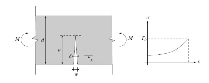
Industrial applications of fibre-reinforced concrete (FRC) in structures require extensive experimental and analytical investigations of the FRC material properties. For design purposes and applications involving the flexural loading of the member, it is essential to have a predictive model for the flexural strength of the FRC material. In the present paper, a fracture mechanics approach based on Bridged Crack Model (BCM) is used to predict the flexural strength of steel fibre-reinforced concrete (SFRC) beams. The model assumes a quadratic tension-softening relationship (σ-δ) governing the bridging action of the steel fibres and a linear profile of the propagating crack. The proposed tension-softening relationship is considered valid for a wide range of fibre-reinforced concrete materials based on the knowledge of either the material micromechanical parameters (such as fibre volume fraction, fibre/matrix bond strength, fibre length, and fibre tensile strength) or an actual experimentally-measured σ-δ relationship. The flexural strength model thus obtained allows the prediction of the flexural strength of SFRC and study the variation of the latter as a function of the micromechanical parameters. An experimental program involving the flexural testing of 13 SFRC prism series was carried out to verify the prediction of the proposed model. The SFRC mixes incorporated two types of steel fibres (straight-end and hooked-end), four different concrete compressive strengths (40, 50, 60, and 70 MPa), three different fibre volume fractions (1, 1.5, and 2%), and three specimen depths (100, 150, and 200 mm). The experimental results were compared to the predictions of the proposed flexural strength model, and a reasonable agreement between the two has been observed. The model provided a useful physical explanation for the observed variation of flexural strength as a function of the test variables investigated in this study.

| [1] |
Li VC, Maalej M (1996) Toughening in cement based composites. Part I: concrete, mortar, and concrete. Cement Concrete Comp 18: 223–237. https://doi.org/10.1016/0958-9465(95)00028-3 doi: 10.1016/0958-9465(95)00028-3

|
| [2] |
Li VC, Maalej M (1996) Toughening in cement based composites. Part Ⅱ: Fiber reinforced cementitious composites. Cement Concrete Comp 18: 239–249. https://doi.org/10.1016/0958-9465(95)00029-1 doi: 10.1016/0958-9465(95)00029-1
|
| [3] |
Hillerborg A, Modéer M, Petersson PE (1976) Analysis of crack formation and crack growth In concrete by means of fracture mechanics and finite elements. Cement Concrete Res 6: 773–781. https://doi.org/10.1016/0008-8846(76)90007-7 doi: 10.1016/0008-8846(76)90007-7
|
| [4] | Hillerborg A (1978) A model for fracture analysis. TVBM-3005. Available from: https://portal.research.lu.se/en/publications/a-model-for-fracture-analysis. |
| [5] | Bažant ZP (1992) Should design codes consider fracture mechanics size effect?, In: Gerstle W, Bazant ZP, Concrete Design Based on Fracture Mechanics, American Concrete Institute, 134: 1–24. |
| [6] | Carpinteri A (1981) A fracture mechanics model for reinforced concrete collapse. Available from: https://www.e-periodica.ch/cntmng?pid=bse-re-001:1981:34::9. |
| [7] |
Carpinteri A (1984) Stability of fracturing process in RC beams. J Struct Eng 110: 544–558. https://doi.org/10.1061/(ASCE)0733-9445(1984)110:3(544) doi: 10.1061/(ASCE)0733-9445(1984)110:3(544)
|
| [8] |
Bazant ZP, Pfeiffer A (1987) Determination of fracture energy from size effect and brittleness number. ACI Mater J 84: 463–480. https://doi.org/10.14359/2526 doi: 10.14359/2526
|
| [9] |
Bažant ZP, Oh BH (1983) Crack band theory for fracture of concrete. Mat Constr 16: 155–177. https://doi.org/10.1007/BF02486267 doi: 10.1007/BF02486267
|
| [10] |
Jenq Y, Shah SP (1985) Two parameter fracture model for concrete. J Eng Mech 111: 1227–1241. https://doi.org/10.1061/(ASCE)0733-9399(1985)111:10(1227) doi: 10.1061/(ASCE)0733-9399(1985)111:10(1227)
|
| [11] |
Xu S, Reinhardt HW (2000) A simplified method for determining double-K fracture parameters for three-point bending tests. Int J Fract 104: 181–209. https://doi.org/10.1023/A:1007676716549 doi: 10.1023/A:1007676716549
|
| [12] |
Xu S, Reinhardt HW (1999) Determination of double-K criterion for crack propagation in quasi-brittle fracture, Part I : Experimental investigation of crack propagation. Int J Frac 98: 111–149. https://doi.org/10.1023/A:1018668929989 doi: 10.1023/A:1018668929989
|
| [13] |
Xu S, Reinhardt HW (1999) Determination of double-K criterion for crack propagation in quasi-brittle fracture, Part Ⅱ : Analytical evaluating and practical measuring methods for three-point bending notched beams. Int J Fract 98: 151–177. https://doi.org/10.1023/A:1018740728458 doi: 10.1023/A:1018740728458
|
| [14] |
Maalej M, Li VC (1995) Flexural strength of fiber cementitious composites. J Materi Civil Eng 6: 390–406. https://doi.org/10.1061/(ASCE)0899-1561(1994)6:3(390) doi: 10.1061/(ASCE)0899-1561(1994)6:3(390)
|
| [15] |
Maalej M, Li VC, Hashida T (1995) Effect of fiber rupture on tensile properties of short fiber composites. J Eng Mech (ASCE) 121: 903. https://doi.org/10.1061/(ASCE)0733-9399(1995)121:8(903) doi: 10.1061/(ASCE)0733-9399(1995)121:8(903)
|
| [16] |
Zhang J, Li VC (2004) Simulation of crack propagation in fiber-reinforced concrete by fracture mechanics. Cem Concr Res 34: 333–339. https://doi.org/10.1016/j.cemconres.2003.08.015 doi: 10.1016/j.cemconres.2003.08.015
|
| [17] |
Accornero F, Rubino A, Carpinteri A (2020) Ductile-to-brittle transition in fiber-reinforced concrete beams: Scale and fiber volume fraction effects. MDPC 2020: 1–11. https://doi.org/10.1002/mdp2.127 doi: 10.1002/mdp2.127
|
| [18] |
Accornero F, Rubino A, Carpinteri A (2022) A fracture mechanics approach to the design of hybrid-reinforced concrete beams. Eng Fract Mech 275: 108821. https://doi.org/10.1016/j.engfracmech.2022.108821 doi: 10.1016/j.engfracmech.2022.108821
|
| [19] | Carpinteri A, Accornero F, Rubino A (2022) Scale effects in the post-cracking behaviour of fibre-reinforced concrete beams. Int J Fract. https://doi.org/10.1007/s10704-022-00671-x |
| [20] |
Accornero F, Rubino A, Carpinteri A (2022) Post-cracking regimes in the flexural behaviour of fibre-reinforced concrete beams. Int J Solids Struct 248: 111637. https://doi.org/10.1016/j.ijsolstr.2022.111637 doi: 10.1016/j.ijsolstr.2022.111637
|
| [21] |
Accornero F, Rubino A, Carpinteri A (2022) Ultra-low cycle fatigue (ULCF) in fibre-reinforced concrete beams. Theor Appl Fract Mec 120: 103392. https://doi.org/10.1016/j.tafmec.2022.103392 doi: 10.1016/j.tafmec.2022.103392
|
| [22] |
Lok TS, Xiao JR (1999) Flexrual strength assessment of fiber reinforced concrete. J Mater Civil Eng 11: 118–196. https://doi.org/10.1061/(ASCE)0899-1561(1999)11:3(188) doi: 10.1061/(ASCE)0899-1561(1999)11:3(188)
|
| [23] |
Meng G, Wu B, Xu S, et al. (2021) Modelling and experimental validation of flexural tensile properties of steel fiber reinforced concrete. Constr Build Mater 273: 121974. https://doi.org/10.1016/j.conbuildmat.2020.121974 doi: 10.1016/j.conbuildmat.2020.121974
|
| [24] |
Zeng JJ, Zeng WB, Ye YY, et al. (2022) Flexural behavior of FRP grid reinforced ultra-high-performance concrete composite plates with different types of fibers. Eng Struct 272: 115020. https://doi.org/10.1016/j.engstruct.2022.115020 doi: 10.1016/j.engstruct.2022.115020
|
| [25] |
Soetens T, Matthys S (2014) Different methods to model the post-cracking behaviour of hooked-end steel fibre reinforced concrete. Constr Build Mater 73: 458–471. https://doi.org/10.1016/j.conbuildmat.2014.09.093 doi: 10.1016/j.conbuildmat.2014.09.093
|
| [26] |
Zhang J, Leung CK, Xu S (2010) Evaluation of fracture parameters of concrete from bending test using inverse analysis approach. Mater Struct 43: 857–874. https://doi.org/10.1617/s11527-009-9552-5 doi: 10.1617/s11527-009-9552-5
|
| [27] |
Da Silva CN, Ciambella J, Barros JAO, et al. (2020) A multiscale model for optimising the flexural capacity of FRC structural elements. Compos Part B-Eng 200: 108325. https://doi.org/10.1016/j.compositesb.2020.108325 doi: 10.1016/j.compositesb.2020.108325
|
| [28] |
Bhosale AB, Prakash SS (2020) Crack propagation analysis of synthetic vs. steel vs. hybrid fibre-reinforced concrete beams using digital image correlation technique. Int J Concr Struct M 14: 1–19. https://doi.org/10.1186/s40069-020-00427-8 doi: 10.1186/s40069-020-00427-8
|
| [29] |
Kravchuk R, Landis EN (2018) Acoustic emission-based classification of energy dissipation mechanisms during fracture of fiber-reinforced ultra-high-performance concrete. Constr Build Mater 176: 531–538. https://doi.org/10.1016/j.conbuildmat.2018.05.039 doi: 10.1016/j.conbuildmat.2018.05.039
|
| [30] |
Chen C, Chen X, Ning Y (2022) Identification of fracture damage characteristics in ultra-high performance cement-based composite using digital image correlation and acoustic emission techniques. Compos Struct 291: 115612. https://doi.org/10.1016/j.compstruct.2022.115612 doi: 10.1016/j.compstruct.2022.115612
|
| [31] |
He F, Biolzi L, Carvelli V, et al. (2022) Digital imaging monitoring of fracture processes in hybrid steel fiber reinforced concrete. Compos Struct 298: 116005. https://doi.org/10.1016/j.compstruct.2022.116005 doi: 10.1016/j.compstruct.2022.116005
|
| [32] | Tada H, Paris PC, Irwin GR (2000) The Stress Analysis of Crack Handbook, 3 Eds., ASME Press. https://doi.org/10.1115/1.801535 |
| [33] |
Ward RJ, Li VC (1991) Dependence of flexural behaviour of fibre reinforced mortar on material fracture resistance and beam size. Constr Build Mater 5: 151–161. https://doi.org/10.1016/0950-0618(91)90066-T doi: 10.1016/0950-0618(91)90066-T
|
| [34] |
Johnston CD (1982) Steel fiber reinforced and plain concrete: factors influencing flexural strength measurement. ACI J Proc 79: 131–138. https://doi.org/10.14359/10888 doi: 10.14359/10888
|
| [35] |
Yoo DY, Banthia N, Yang JM, et al. (2016) Size effect in normal- and high-strength amorphous metallic and steel fiber reinforced concrete beams. Constr Build Mater 121: 676–685. https://doi.org/10.1016/j.conbuildmat.2016.06.040 doi: 10.1016/j.conbuildmat.2016.06.040
|
| [36] |
Li VC, Wang Y, Backer S (1900) Effect of inclining angle, bundling and surface treatment on synthetic fibre pull-out from a cement matrix. Composites 21: 132–140. https://doi.org/10.1016/0010-4361(90)90005-H doi: 10.1016/0010-4361(90)90005-H
|
| [37] |
Ince R (2012) Determination of concrete fracture parameters based on peak-load method with diagonal split-tension cubes. Eng Fract Mech 82: 100–114. https://doi.org/10.1016/j.engfracmech.2011.11.026 doi: 10.1016/j.engfracmech.2011.11.026
|
| [38] |
Chbani H, Saadouki B, Boudlal M, et al. (2019) Determination of fracture toughness in plain concrete specimens by R curve. Frat Integrita Strut 13: 763–774. https://doi.org/10.3221/IGF-ESIS.49.68 doi: 10.3221/IGF-ESIS.49.68
|
| [39] |
Xu S, Zhang X (2008) Determination of fracture parameters for crack propagation in concrete using an energy approach. Eng Fract Mech 75: 4292–4308. https://doi.org/10.1016/j.engfracmech.2008.04.022 doi: 10.1016/j.engfracmech.2008.04.022
|
| [40] | British Standards Institution (2007) Structural use of concrete-part 1 : code of practice for design and construction. Available from: https://crcrecruits.files.wordpress.com/2014/04/bs8110-1-1997-structural-use-of-concrete-design-construction.pdf |
| [41] |
Lee J, Cho B, Choi E (2017) Flexural capacity of fiber reinforced concrete with a consideration of concrete strength and fiber content. Constr Build Mater 138: 222–231. https://doi.org/10.1016/j.conbuildmat.2017.01.096 doi: 10.1016/j.conbuildmat.2017.01.096
|
| [42] |
Yoo DY, Yoon YS, Banthia N (2015) Flexural response of steel-fiber-reinforced concrete beams: Effects of strength, fiber content, and strain-rate. Cement Concrete Compos 64: 84–92. https://doi.org/10.1016/j.cemconcomp.2015.10.001 doi: 10.1016/j.cemconcomp.2015.10.001
|
| [43] |
Jang SJ, Jeong GY, Lee MH, et al. (2016) Compressive strength effects on flexural behavior of steel fiber reinforced concrete. Key Eng Mater 709: 101–104. https://doi.org/10.4028/www.scientific.net/KEM.709.101 doi: 10.4028/www.scientific.net/KEM.709.101
|
| [44] | Soutsos M, Domone P (2017) Construction Materials: Their Nature and Behaviour, CRC Press. https://doi.org/10.1201/9781315164595 |


Figures(11) / Tables(3)

Abdul Saboor Karzad, Moussa Leblouba, Zaid A. Al-Sadoon, Mohamed Maalej, Salah Altoubat. Modeling the flexural strength of steel fibre reinforced concrete[J]. AIMS Materials Science, 2023, 10(1): 86-111. doi: 10.3934/matersci.2023006


 DownLoad: