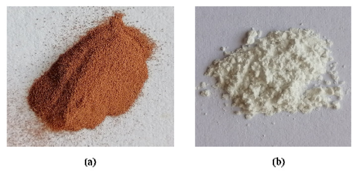
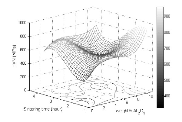
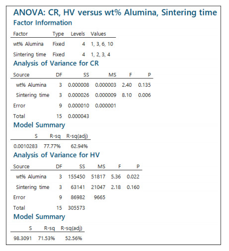
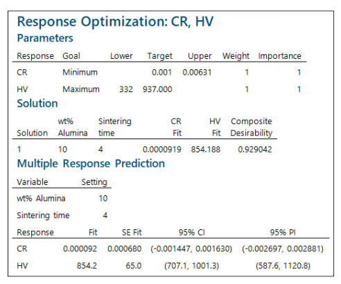
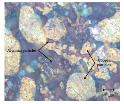
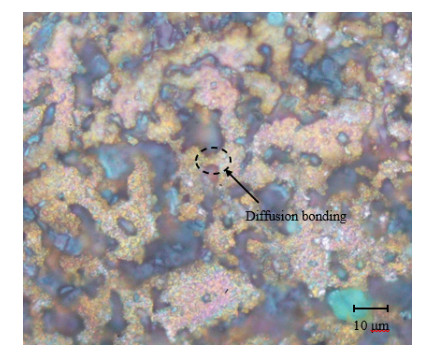
Copper alumina (Cu-x%Al2O3) was prepared from micro-sized powder particles through the powder metallurgy (PM) process. Experimental runs were designed according to the design of experiments (DOE) methodology to investigate the effect of alumina concentration and sintering time on the hardness and corrosion rate of the powdered composite. Four sintering times were tested (1, 2, 3, and 4 h) in combination with different levels of alumina concentration (1 wt%, 3 wt%, 6 wt%, and 10 wt%). Given the narrow range of the sintering temperature for copper alumina, this temperature was fixed at 900 ℃, whereas the compaction pressure was set at 300 MPa. Collected data were analysed based on the analysis of variance (ANOVA) approach and complemented with microscopic analysis. Optimization techniques were used to identify the optimal settings of sintering time and alumina concentration for the PM composite.
Citation: Omar Bataineh, Abdullah F. Al-Dwairi, Zaid Ayoub, Mohammad Al-Omosh. DOE-based experimental investigation and optimization of hardness and corrosion rate for Cu-x%Al2O3 as processed by powder metallurgy[J]. AIMS Materials Science, 2021, 8(3): 416-433. doi: 10.3934/matersci.2021026
Copper alumina (Cu-x%Al2O3) was prepared from micro-sized powder particles through the powder metallurgy (PM) process. Experimental runs were designed according to the design of experiments (DOE) methodology to investigate the effect of alumina concentration and sintering time on the hardness and corrosion rate of the powdered composite. Four sintering times were tested (1, 2, 3, and 4 h) in combination with different levels of alumina concentration (1 wt%, 3 wt%, 6 wt%, and 10 wt%). Given the narrow range of the sintering temperature for copper alumina, this temperature was fixed at 900 ℃, whereas the compaction pressure was set at 300 MPa. Collected data were analysed based on the analysis of variance (ANOVA) approach and complemented with microscopic analysis. Optimization techniques were used to identify the optimal settings of sintering time and alumina concentration for the PM composite.

| [1] |
Alem SAA, Latifi R, Angizi S, et al. (2020) Microwave sintering of ceramic reinforced metal matrix composites and their properties: a review. Mater Manuf Process 35: 303-327. doi: 10.1080/10426914.2020.1718698

|
| [2] |
Sankar S, Naik AA, Anilkumar T, et al. (2020) Characterization, conductivity studies, dielectric properties, and gas sensing performance of in situ polymerized polyindole/copper alumina nanocomposites. J Appl Polym Sci 137: 49145. doi: 10.1002/app.49145
|
| [3] | Singh G, Singh S, Singh J, et al. (2020) Parameters effect on electrical conductivity of copper fabricated by rapid manufacturing. Mater Manuf Process 1-12. |
| [4] |
Asano K (2015) Preparation of alumina fiber-reinforced aluminum by squeeze casting and their machinability. Mater Manuf Process 30: 1312-1316. doi: 10.1080/10426914.2015.1019101
|
| [5] |
Strojny-Nędza A, Pietrzak K, Gili F, et al. (2020) FGM based on copper-alumina composites for brake disc applications. Arch Civ Mech Eng 20: 83. doi: 10.1007/s43452-020-00079-1
|
| [6] |
Mohamad SNS, Mahmed N, Halin DSC, et al. (2019) Synthesis of alumina nanoparticles by sol-gel method and their applications in the removal of copper ions (Cu2+) from the solution. IOP Conf Ser: Mater Sci Eng 701: 12034. doi: 10.1088/1757-899X/701/1/012034
|
| [7] |
Tang Y, Qiu S, Li M, et al. (2017) Fabrication of alumina/copper heat dissipation substrates by freeze tape casting and melt infiltration for high-power LED. J Alloy Compd 690: 469-477. doi: 10.1016/j.jallcom.2016.08.149
|
| [8] | Duan L, Jiang H, Zhang X, et al. (2020) Experimental investigations of electromagnetic punching process in CFRP laminate. Mater Manuf Process 1-12. |
| [9] |
Sang K, Weng Y, Huang Z, et al. (2016) Preparation of interpenetrating alumina-copper composites. Ceram Int 42: 6129-6135. doi: 10.1016/j.ceramint.2015.12.174
|
| [10] |
Winzer J, Weiler L, Pouquet J, et al. (2011) Wear behaviour of interpenetrating alumina-copper composites. Wear 271: 2845-2851. doi: 10.1016/j.wear.2011.05.042
|
| [11] |
Rakoczy J, Nizioł J, Wieczorek-Ciurowa K, et al. (2013) Catalytic characteristics of a copper-alumina nanocomposite formed by the mechanochemical route. React Kinet Mech Cat 108: 81-89. doi: 10.1007/s11144-012-0503-8
|
| [12] | Rajesh kumar L, Amirthagadeswaran KS (2019) Corrosion and wear behaviour of nano Al2O3 reinforced copper metal matrix composites synthesized by high energy ball milling. Particulate Science and Technology 1-8. |
| [13] |
Eddine WZ, Matteazzi P, Celis JP (2013) Mechanical and tribological behavior of nanostructured copper-alumina cermets obtained by pulsed electric current sintering. Wear 297: 762-773. doi: 10.1016/j.wear.2012.10.011
|
| [14] |
Mohammadi E, Nasiri H, Khaki JV, et al. (2018) Copper-alumina nanocomposite coating on copper substrate through solution combustion. Ceram Int 44: 3226-3230. doi: 10.1016/j.ceramint.2017.11.094
|
| [15] |
Wang X, Ma J, Maximenko A, et al. (2005) Sequential deposition of copper/alumina composites. J Mater Sci 40: 3293-3295. doi: 10.1007/s10853-005-2704-2
|
| [16] |
Lim JD, Susan YSY, Daniel RM, et al. (2013) Surface roughness effect on copper-alumina adhesion. Microelectron Reliab 53: 1548-1552. doi: 10.1016/j.microrel.2013.07.016
|
| [17] |
Qiao Y, Cai X, Zhou L, et al. (2018) Microstructure and mechanical properties of copper matrix composites synergistically reinforced by Al2O3 and CNTs. Integr Ferroelectr 191: 133-144. doi: 10.1080/10584587.2018.1457383
|
| [18] |
Sadoun A, Ibrahim A, Abdallah AW (2020) Fabrication and evaluation of tribological properties of Al2O3 coated Ag reinforced copper matrix nanocomposite by mechanical alloying. J Asian Ceram Soc 8: 1228-1238. doi: 10.1080/21870764.2020.1841073
|
| [19] |
Rajkovic V, Bozic D, Stasic J, et al. (2014) Processing, characterization and properties of copper-based composites strengthened by low amount of alumina particles. Powder Technol 268: 392-400. doi: 10.1016/j.powtec.2014.08.051
|
| [20] |
Yousif AA, Moustafa SF, El-Zeky MA, et al. (2003) Alumina particulate/Cu matrix composites prepared by powder metallurgy. Powder Metall 46: 307-311. doi: 10.1179/00325890322500849
|
| [21] |
Korać M, Kamberović Ž, Anđić Z, et al. (2010) Sintered materials based on copper and alumina powders synthesized by a novel method. Sci Sinter 42: 81-90. doi: 10.2298/SOS1001081K
|
| [22] |
Zheng Z, Li XJ, Gang T (2009) Manufacturing nano-alumina particle-reinforced copper alloy by explosive compaction. J Alloy Compd 478: 237-239. doi: 10.1016/j.jallcom.2008.12.008
|
| [23] |
Yousefieh M, Shamanian M, Arghavan AR (2012) Analysis of design of experiments methodology for optimization of pulsed current GTAW process parameters for ultimate tensile strength of UNS S32760 welds. Metallogr Microstr Anal 1: 85-91. doi: 10.1007/s13632-012-0017-9
|
| [24] | Bataineh O, Al-shoubaki A, Barqawi O (2012) Optimising process conditions in MIG welding of aluminum alloys through factorial design experiments. Latest Trends in Environmental and Manufacturing Engineering Optimising 21-26. |
| [25] |
Thiraviam R, Sornakumar T, Senthil Kumar A (2008) Development of copper: alumina metal matrix composite by powder metallurgy method. Int J Mater Prod Tec 31: 305-313. doi: 10.1504/IJMPT.2008.018029
|
| [26] | Montgomery DC (2017) Design and Analysis of Experiments, 9 Eds., Hoboken: John Wiley & Sons. |
| [27] | Bataineh O (2019) Effect of roller burnishing on the surface roughness and hardness of 6061-T6 aluminum alloy using ANOVA. IJMERR 8: 565-569. |
| [28] |
Bataineh O, Dalalah D (2010) Strategy for optimising cutting parameters in the dry turning of 6061-T6 aluminium alloy based on design of experiments and the generalised pattern search algorithm. IJMMM 7: 39-57. doi: 10.1504/IJMMM.2010.029845
|
| [29] |
Equbal MI, Equbal A, Mukerjee D (2018) A full factorial design-based desirability function approach for optimization of hot forged vanadium micro-alloyed steel. Metallogr Microsta Anal 7: 504-523. doi: 10.1007/s13632-018-0473-y
|
| [30] |
Almomani MA, Tyfour WR, Nemrat MH (2016) Effect of silicon carbide addition on the corrosion behavior of powder metallurgy Cu-30Zn brass in a 3.5 wt% NaCl solution. J Alloy Compd 679: 104-114. doi: 10.1016/j.jallcom.2016.04.006
|
| [31] |
Michálek M, Sedláček J, Parchoviansky M, et al. (2014) Mechanical properties and electrical conductivity of alumina/MWCNT and alumina/zirconia/MWCNT composites. Ceram Int 40: 1289-1295. doi: 10.1016/j.ceramint.2013.07.008
|
| [32] | Yoshino Y (1989) Role of oxygen in bonding copper to alumina. J Am Ceram Soc 27: 1322-1327. |
| [33] |
Hu W, Donat F, Scott SA, et al. (2016) The interaction between CuO and Al2O3 and the reactivity of copper aluminates below 1000 ℃ and their implication on the use of the Cu-Al-O system for oxygen storage and production. RSC Adv 6: 113016-113024. doi: 10.1039/C6RA22712K
|
Figures(14) / Tables(2)

Omar Bataineh, Abdullah F. Al-Dwairi, Zaid Ayoub, Mohammad Al-Omosh. DOE-based experimental investigation and optimization of hardness and corrosion rate for Cu-x%Al2O3 as processed by powder metallurgy[J]. AIMS Materials Science, 2021, 8(3): 416-433. doi: 10.3934/matersci.2021026


 DownLoad: